9 Stochastic Processes
9.1 Poisson processes
A Poisson process with intensity \(\lambda\) on the interval \([a, b]\) is generated by simply first generating a Poisson random variable with mean \(\lambda (b-a)\), and then generating an iid sample of that size from the uniform distribution on \([a, b]\).
lambda = 1
a = 0
b = 50
N = rpois(1, lambda*b)
x = runif(N, a, b)
plot(x, rep(1, N), type = "h", xlab = "", ylab = "", axes = FALSE)
axis(1, at = c(a, b))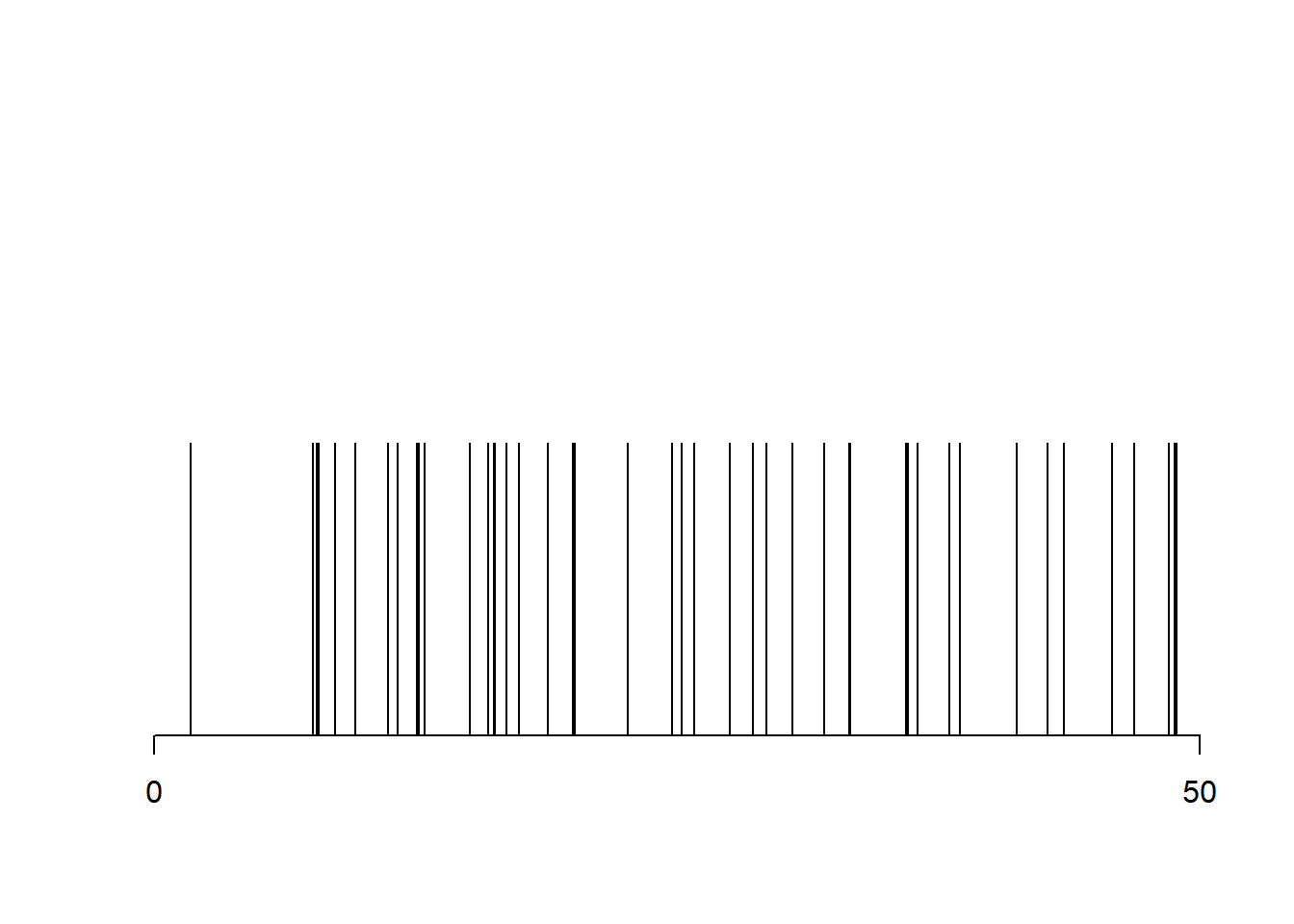
The same process can be generated by producing an infinite iid sequence from the exponential distribution with rate \(\lambda\), computing its partial sums, and returning those that fall in \([a, b]\).
x = a + rexp(1, lambda)
i = 1
while (x[i] < b){
  x = c(x, x[i] + rexp(1, lambda))
  i = i + 1
}
plot(x, rep(1, length(x)), type = "h", xlab = "", ylab = "", axes = FALSE)
axis(1, at = c(a, b))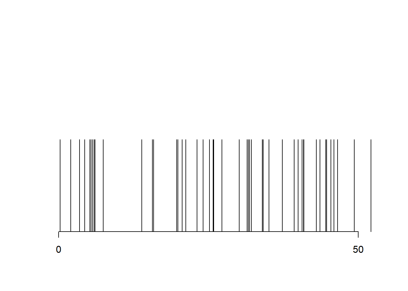
In dimension \(d=2\), a Poisson process with intensity \(\lambda\) on a subset \(\mathcal{D} \subset \mathbb{R}^2\) can be obtained by first generating a Poisson random variable with mean \(\lambda\), and then generating an iid sample of that size from the uniform distribution on \(\mathcal{D}\). We consider the case of an axis-aligned rectangle.
n = 100 # sample size
x = cbind(3*runif(n), runif(n))
plot(x, pch = 16, xlab = "", ylab = "", asp = 1)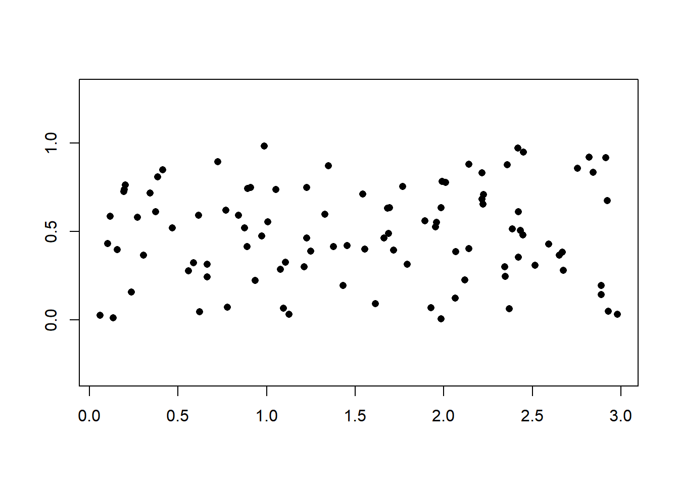
9.2 Markov chains
We start with a two-state Markov chain with transition matrix.
a = 0.5 # probability of staying in state 1
b = 0.1 # probability of staying in state 2
Theta = matrix(c(a, 1-b, 1-a, b), 2, 2) # transition matrix
n = 10 # number of states
x = integer(n+1) # stores the successive states
x[1] = sample(1:2, 1) # starting state drawn uniformly at random
for (i in 1:n){
  x[i+1] = ifelse(x[i] == 1, sample(1:2, prob = c(a, 1-a)), sample(1:2, prob = c(1-b, b)))
}
print(x)
[1] 2 1 2 1 2 1 1 1 2 1 2plot(0:n, x, type = "b", pch = 15, lty = 2, xlab = "time", ylab = "state", axes = FALSE)
axis(1, at = 0:n)
axis(2, at = 1:2)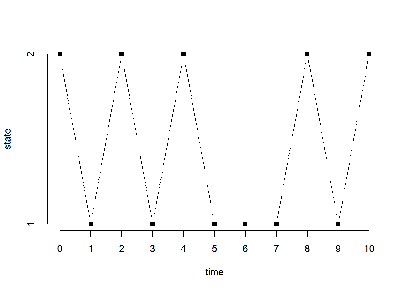
The package allows for the definition of Markov chain objects. We define the same Markov chain (same transition matrix), but change the states to \(A\) and \(B\) (instead of 1 and 2).
require(markovchain)
MC = new("markovchain", states = c("A", "B"), transitionMatrix = Theta)
plot(MC)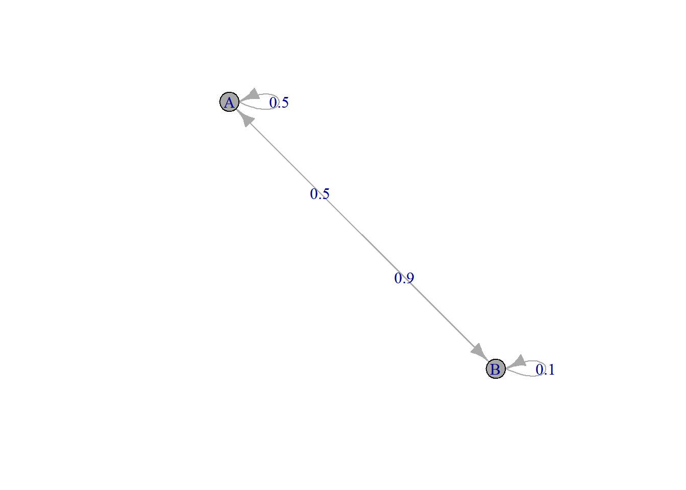
The following generates a sample of size \(n\) from the chain starting at a state that is generated uniformly at random (default).
[1] B A A B A A B A A B Ax[x == "A"] = 1
x[x == "B"] = 2
plot(0:n, x, type = "b", pch = 15, lty = 2, xlab = "time", ylab = "state", axes = FALSE)
axis(1, at = 0:n)
axis(2, at = 1:2, labels = c("A", "B"))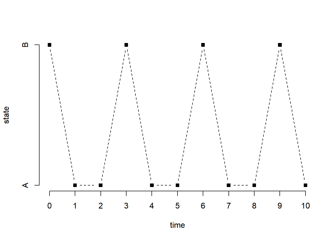
An irreducible, aperiodic, and positively recurrent markov chain has a unique stationary distribution given by the (unique) left eigenvector of the transition matrix for the eigenvalue 1. The chain above satisfies these properties, and its stationary distribution is the following.
out = eigen(t(Theta)) # eigenvalue decomposition of the transpose of the transition matrix
out = out$vec[, 1] # eigenvector corresponding to the eigenvalue 1 (always the top one)
q = as.vector(out)/sum(out) # normalized so the entries sum to 1
names(q) = c("A", "B")
print(q)
A B
0.6428571 0.3571429 This is what the theory says. We can verify that this is indeed the case by running the chain for a long time and compute the fraction of time the run spends in each state.
x
      A       B
0.64277 0.35723
x
A B
0.642855 0.357145 9.3 Simple random walk
A (symmetric) simple random walk is, in a sense, a Markov chain with states \(\{-1, 1\}\), except that the focus is on the partial sums.
n = 1e4 # length of the walk
x = sample(c(-1,1), n, replace = TRUE)
s = c(0, cumsum(x)) # partial sums
plot(0:n, s, type = "l", lwd = 2, xlab = "step", ylab = "partial sum")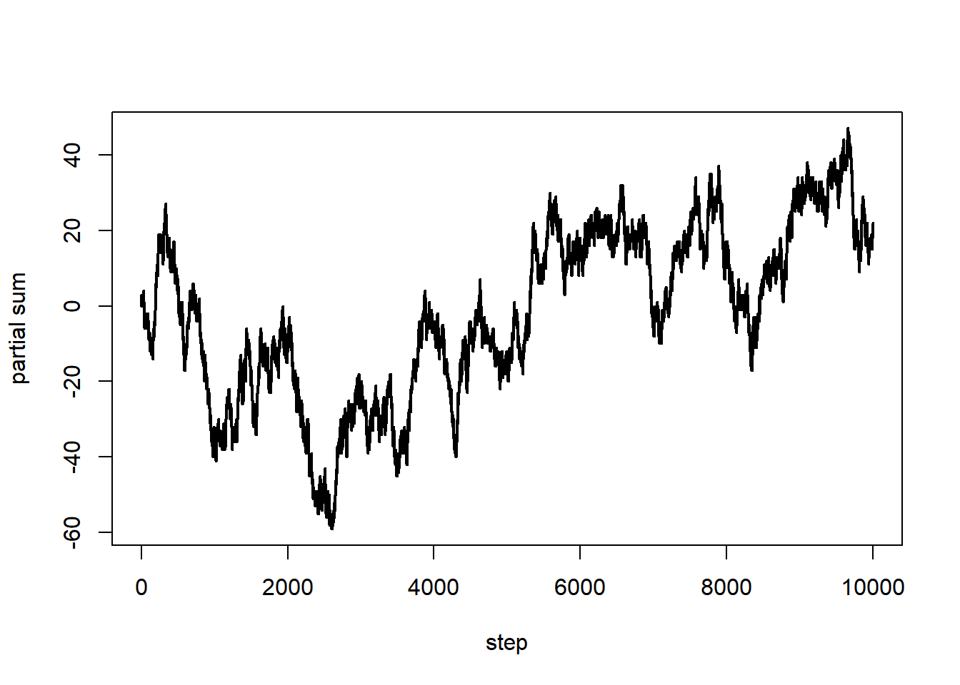
The following is an attempt to verify the result of Erd"os and R'enyi (closely related to the so-called Law of Iterated Logarithm). We plot the normalized partial sums, their cumulative maxima, and what the result predicts.
t = s[-1]/sqrt(1:n) # normalized partial sums
plot(1:n, t, type = "l", lwd = 1, xlab = "step", ylab = "normalized partial sum", ylim = c(min(t), max(max(t), sqrt(2*log(log(n))))))
lines(1:n, cummax(t), lwd = 1, lty = 2)
lines(3:n, sqrt(2*log(log(3:n))), lty = 3)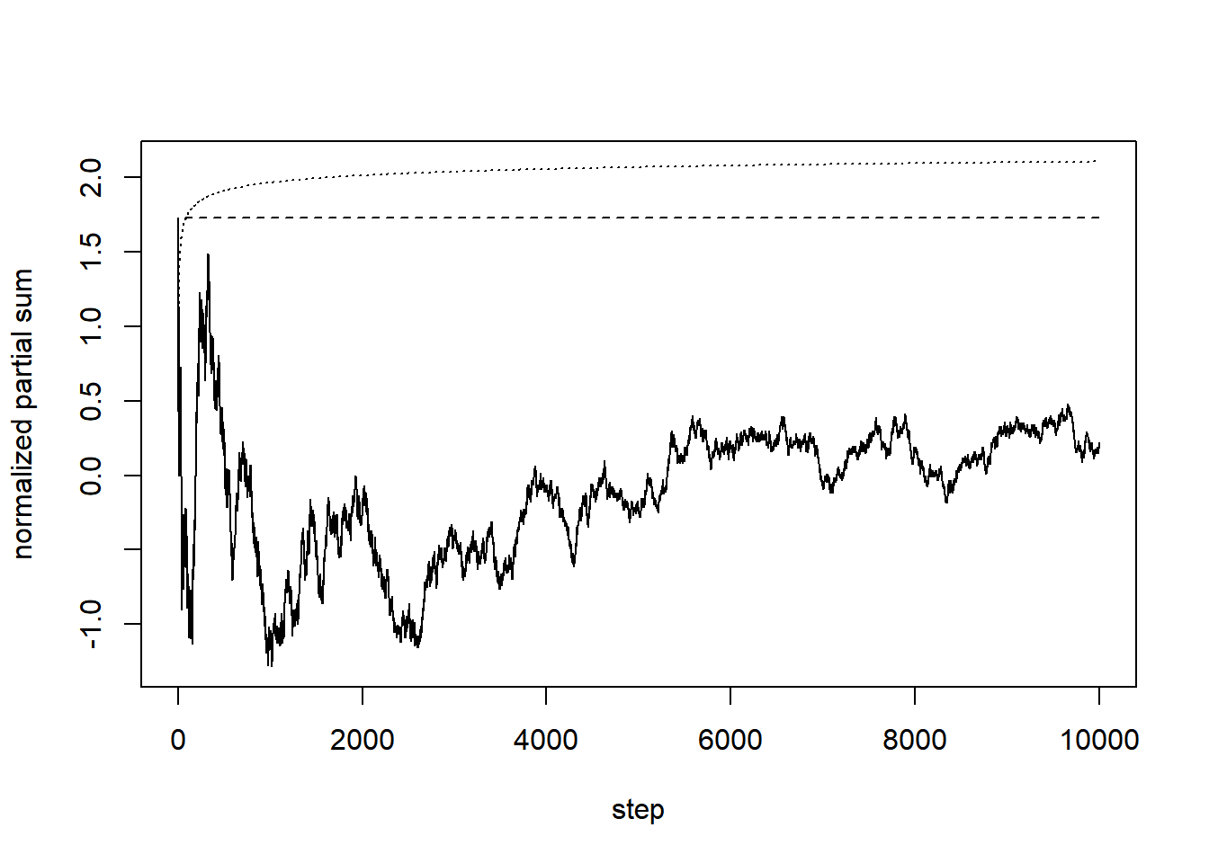
The convergence is very slow, and not particularly obvious in this simulation. It also happens that, most of the time, the maximum happens near the beginning of the normalized partial sum sequence (and this can be proved to be the case in a certain sense).
9.4 Galton–Watson processes
We work with a Poisson offspring distribution, as this is one of the most commonly studied example. The simple code below generates a realization of the sequence of total number of individuals. It does not generates a fully detailed realization (which would have a tree structure).
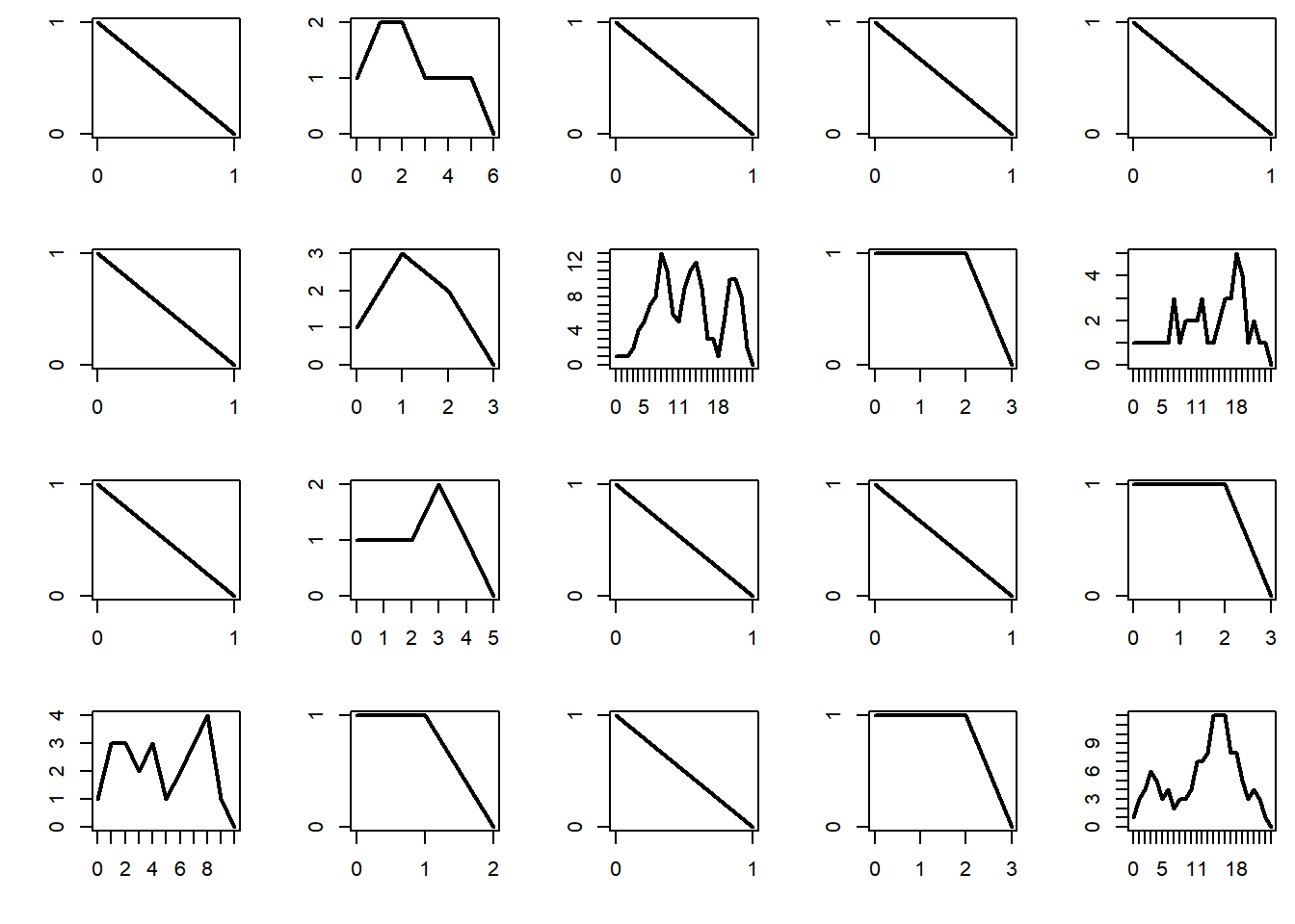
The probability of extinction is 1 if the mean number of offsprings per individual is \(\mu \le 1\), and is strictly positive if \(\mu > 1\). Below we plot the total population per generation for 20 different realizations of the process, and plot them. The subcritical regime corresponds to \(\mu < 1\). In that case, the process dies very quickly.
par(mfrow = c(4, 5), mai = c(0.5, 0.5, 0.1, 0.1))
mu = 0.9
n = 200 # maximum number of generations
for (b in 1:20){
  x = rep(0, n+1)
  x[1] = 1
  for (i in 1:n){
    x[i+1] = sum(rpois(x[i], mu))
    if (x[i+1] == 0) break
    if (x[i+1] > 1e5) break
  }
plot(0:i, x[1:(i+1)], type = "l", lwd = 2, xlab = "", ylab = "", axes = FALSE)
box()
axis(1, at = 0:i)
axis(2, at = 0:max(x))
} 
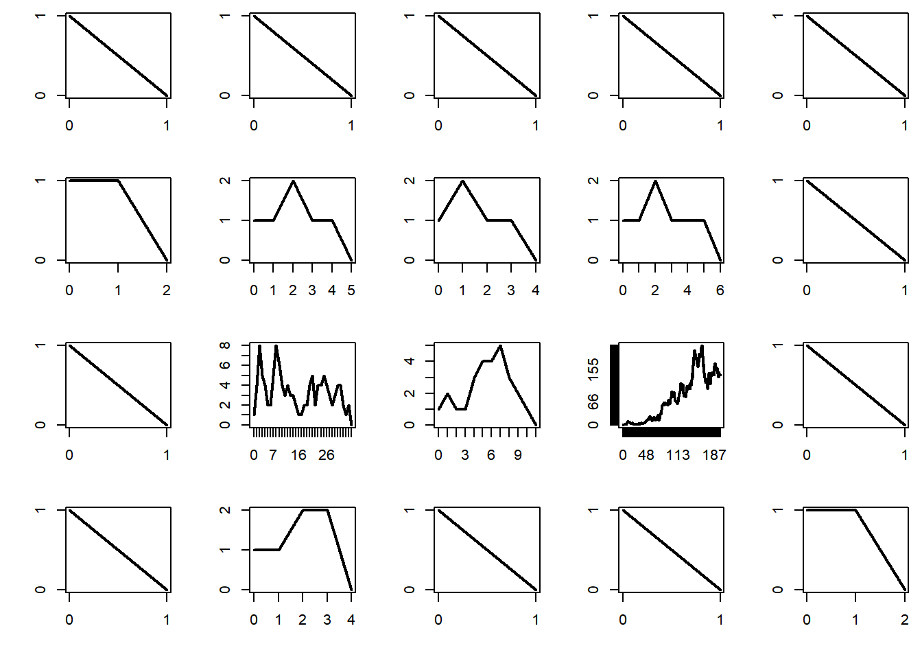
The critical regime corresponds to \(\mu = 1\). In that case the process dies eventually, but on occasion it will survive a relatively long time.
par(mfrow = c(4, 5), mai = c(0.5, 0.5, 0.1, 0.1))
mu = 1
n = 200 # maximum number of generations
for (b in 1:20){
  x = rep(0, n+1)
  x[1] = 1
  for (i in 1:n){
    x[i+1] = sum(rpois(x[i], mu))
    if (x[i+1] == 0) break
    if (x[i+1] > 1e5) break
  }
  plot(0:i, x[1:(i+1)], type = "l", lwd = 2, xlab = "", ylab = "", axes = FALSE)
  box()
  axis(1, at = 0:i)
  axis(2, at = 0:max(x))
} 
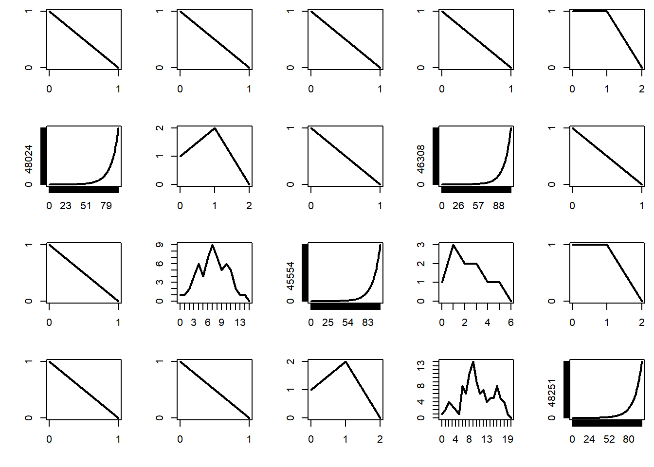
The supercritical regime corresponds to \(\mu > 1\). In that case, the probability that the process survives indefinitely is strictly positive. In addition, it turns out that, when the process survives it increases in size exponentially — and this causes trouble when performing simulations.
par(mfrow = c(4, 5), mai = c(0.5, 0.5, 0.1, 0.1))
mu = 1.1
n = 200 # maximum number of generations
for (b in 1:20){
  x = rep(0, n+1)
  x[1] = 1
  for (i in 1:n){
    x[i+1] = sum(rpois(x[i], mu))
    if (x[i+1] == 0) break
    if (x[i+1] > 1e5) break
  }
  plot(0:i, x[1:(i+1)], type = "l", lwd = 2, xlab = "", ylab = "", axes = FALSE)
  box()
  axis(1, at = 0:i)
  axis(2, at = 0:max(x))
} 
9.5 Random graph models
We use the package, which offers a comprehensive set of functions to generate and manipulate a variety of random graph models and extract statistics from a graph (or network).
9.5.1 Gilbert and Erdos–Renyi random graphs
We examine the distribution of the sizes of the connected components of the graph. The number of nodes is \(n\), and the probability of connection is \(p= \lambda/n\), where we take \(\lambda > 0\) fixed. The subcritical regime corresponds to \(\lambda < 1\).
n = 1e6
lambda = 0.9
p = lambda/n
G = sample_gnp(n, p) # a realization of the random graph model
C = components(G) # connected components
tab = tabulate(C$csize)
plot(tab, type = "h", lwd = 5, log = "xy", xlab = "component size", ylab = "frequency", main = "", col = "darkgrey") # distribution of the sizes of the connected components
abline(h = 1, lty = 3)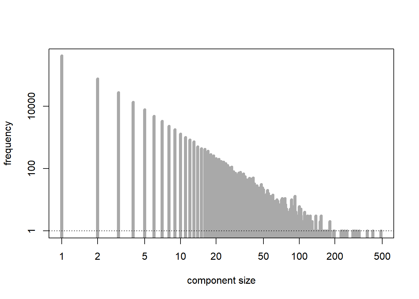
[1] 488[1] 550053The critical regime corresponds to \(\lambda = 1\).
n = 1e6
lambda = 1
p = lambda/n
G = sample_gnp(n, p) # a realization of the random graph model
C = components(G) # connected components
tab = tabulate(C$csize)
plot(tab, type = "h", lwd = 5, log = "xy", xlab = "component size", ylab = "frequency", main = "", col = "darkgrey") # distribution of the sizes of the connected components
abline(h = 1, lty = 3)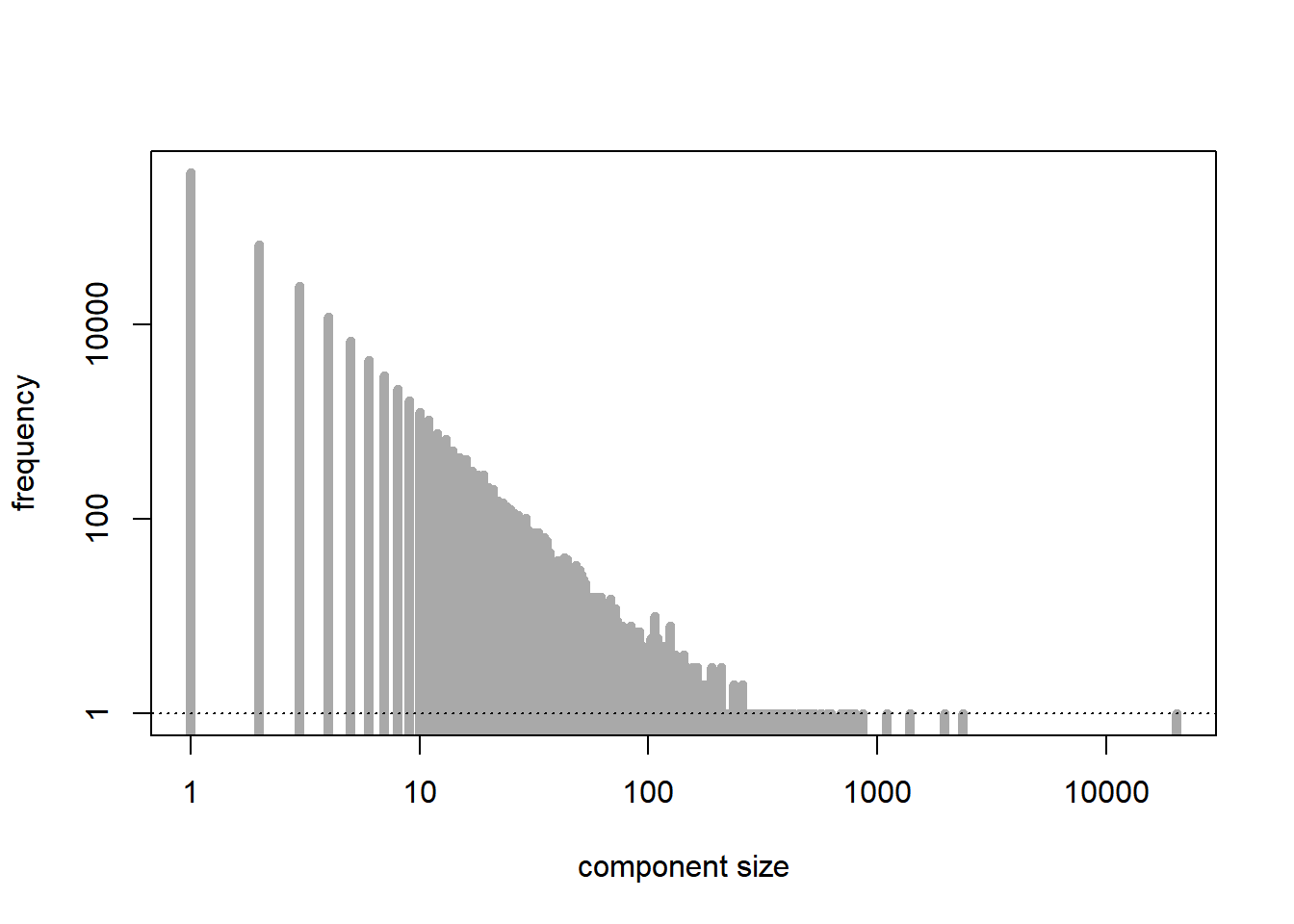
[1] 20304[1] 499750The supercritical regime corresponds to \(\lambda > 1\). As predicted by the theory, except for the largest connected component, which is relatively large, the other connected components are quite small in size.
n = 1e6
lambda = 1.1
p = lambda/n
G = sample_gnp(n, p) # a realization of the random graph model
C = components(G) # connected components
tab = tabulate(C$csize)
plot(tab, type = "h", lwd = 5, log = "xy", xlab = "component size", ylab = "frequency", main = "", col = "darkgrey") # distribution of the sizes of the connected components
abline(h = 1, lty = 3)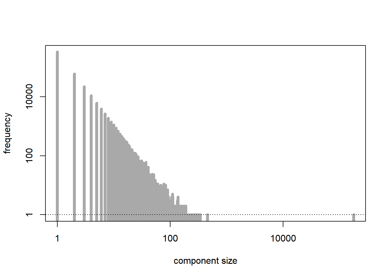
[1] 178789[1] 4496999.5.2 Percolation models
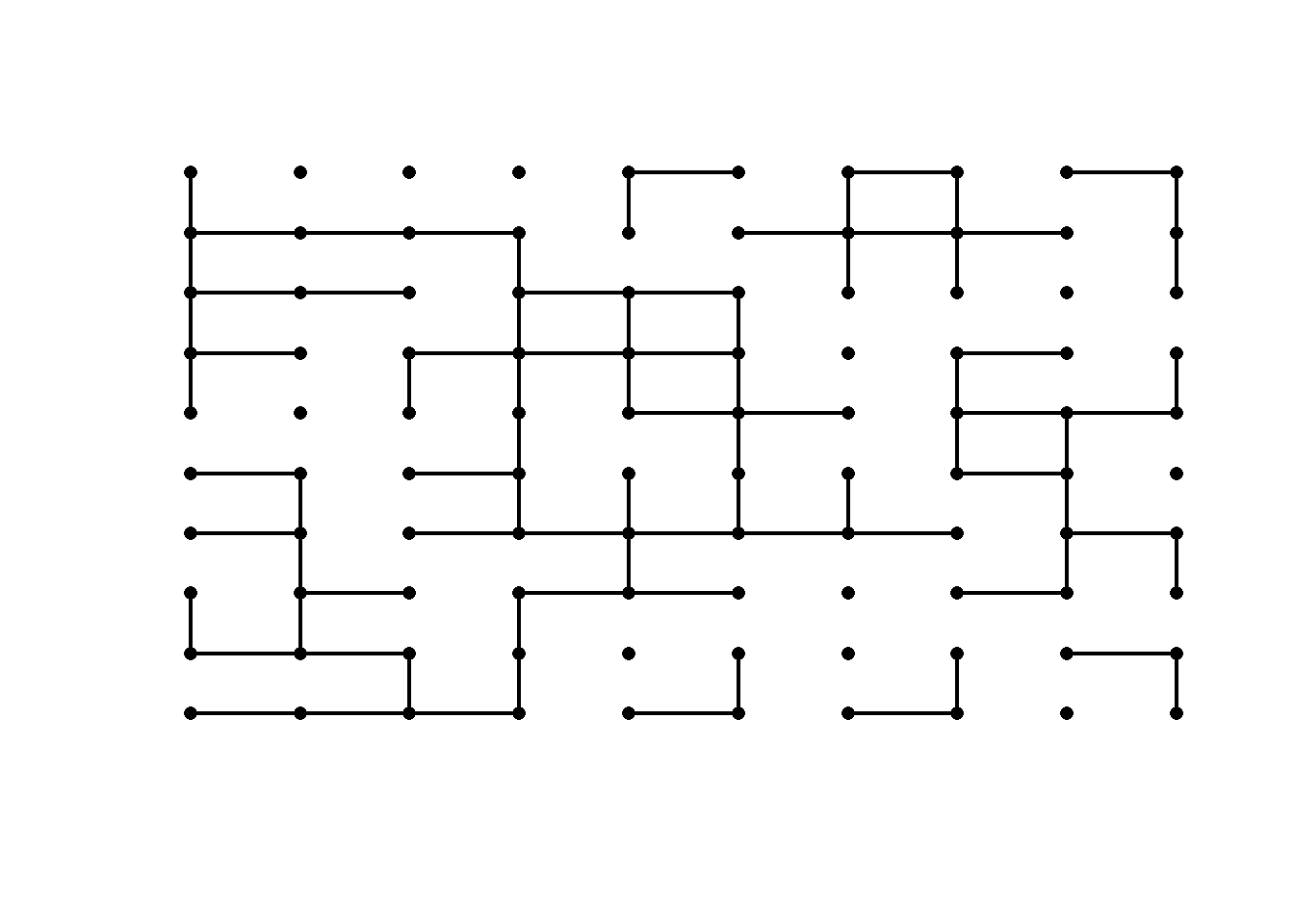
We generate a bond percolation model on the \(n\)-by-\(n\) square lattice, with probability of connection \(p\). Play around with the value of \(p\) to see how a realization of the graph looks like in the subcritical, critical, and supercritical regimes.
p = 0.5 # critical regime
n = 10
x = cbind(gl(n, n), rep(1:n, n))
plot(x, type = "p", axes = FALSE, pch = 16, xlab = "", ylab = "")
for (i in 1:n){
  for (j in 2:n){
    if (rbinom(1, 1, p) == 1)
      lines(c(i, i), c(j-1, j), lwd = 2)
    if (rbinom(1, 1, p) == 1)
      lines(c(j-1, j), c(i, i), lwd = 2)
  }
}
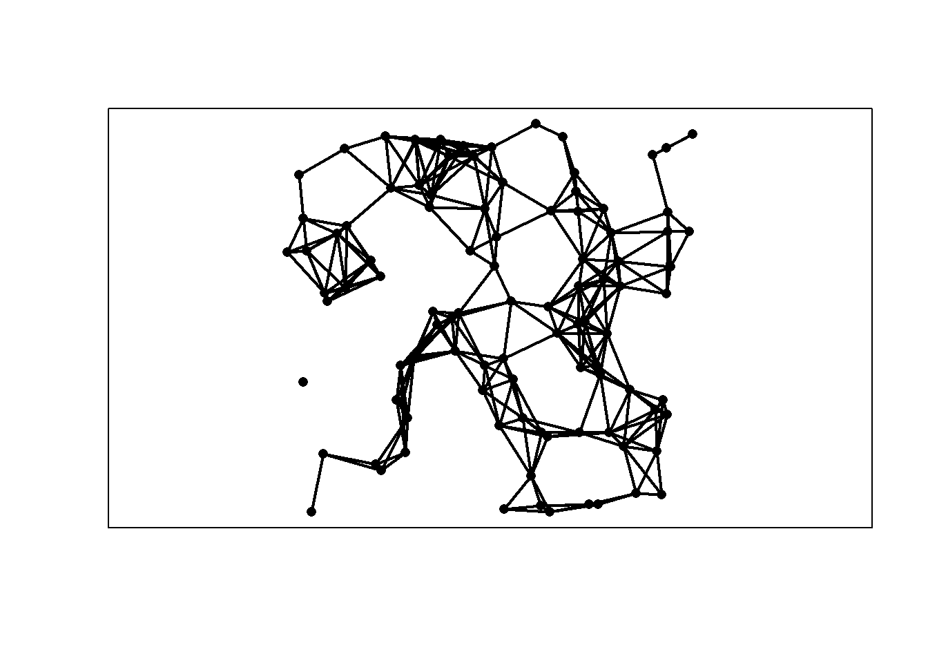
9.5.3 Random geometric graph
We generate a random geometric graph on the unit square based on a sample of size \(n\) from the uniform distribution and connecting every two points that are within distance \(r\) of each other.
r = 0.15
n = 100
x = cbind(runif(n), runif(n))
plot(x, type = "p", axes = FALSE, pch = 16, xlab = "", ylab = "", asp = 1)
box()
D = as.matrix(dist(x))
for (i in 1:(n-1)){
  for (j in 2:n){
    if (D[i, j] <= r)
      lines(x[c(i,j),], lwd = 2)
  }
}