21 Regression Analysis

21.1 Regression

We use simulated data, so that we know the underlying function.

f = function(x) {
  (1 + 10*x - 5*x^2)*sin(10*x)
} # target function

curve(f, lwd = 2)

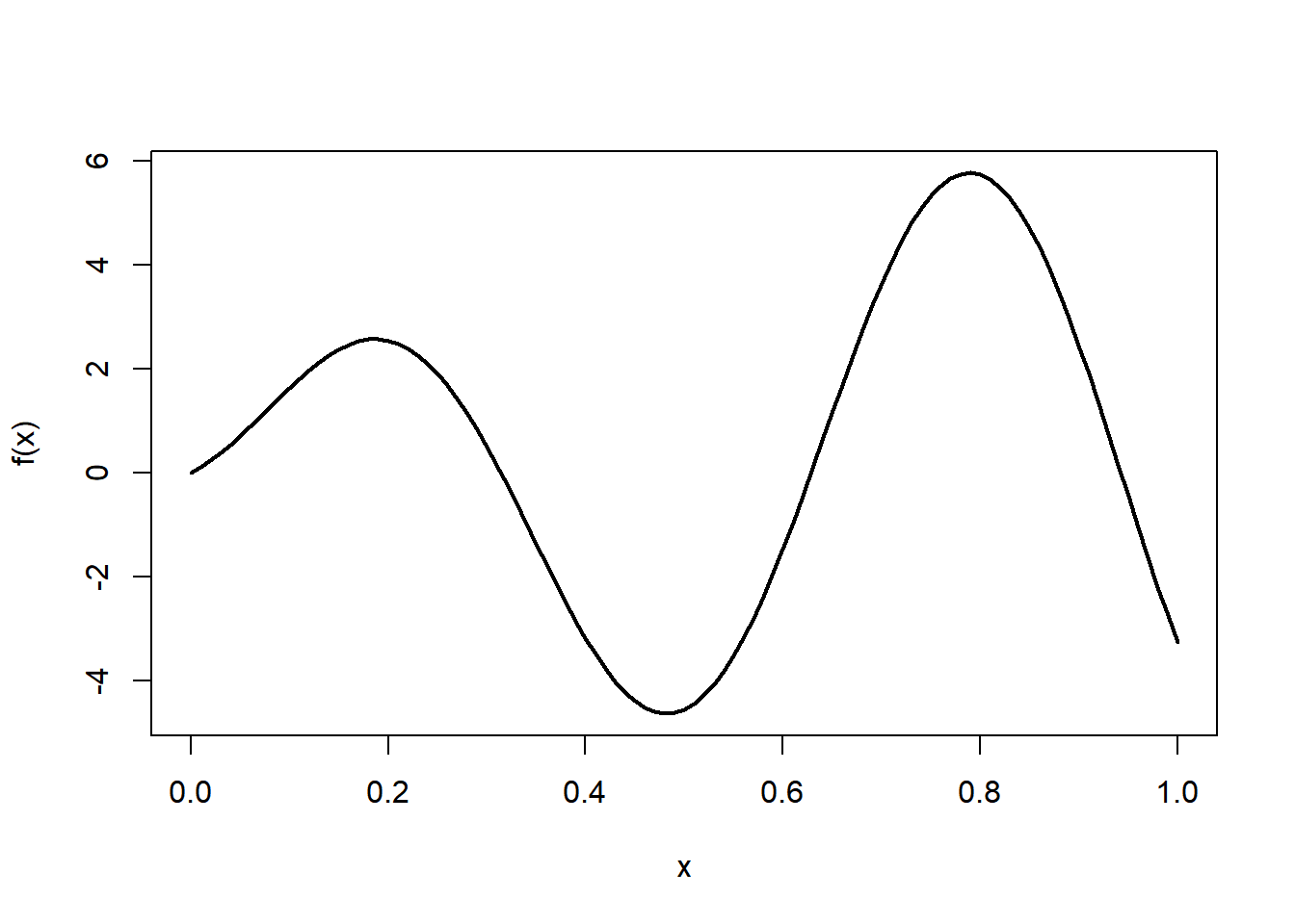
n = 200 # sample size
x = runif(n) # the predictor variable
x = sort(x) # we sort x for ease of plotting
y = f(x) + 0.5*rnorm(n) # the response variable

plot(x, y, pch = 16, col = "darkgrey")
curve(f, lty = 2, add = TRUE)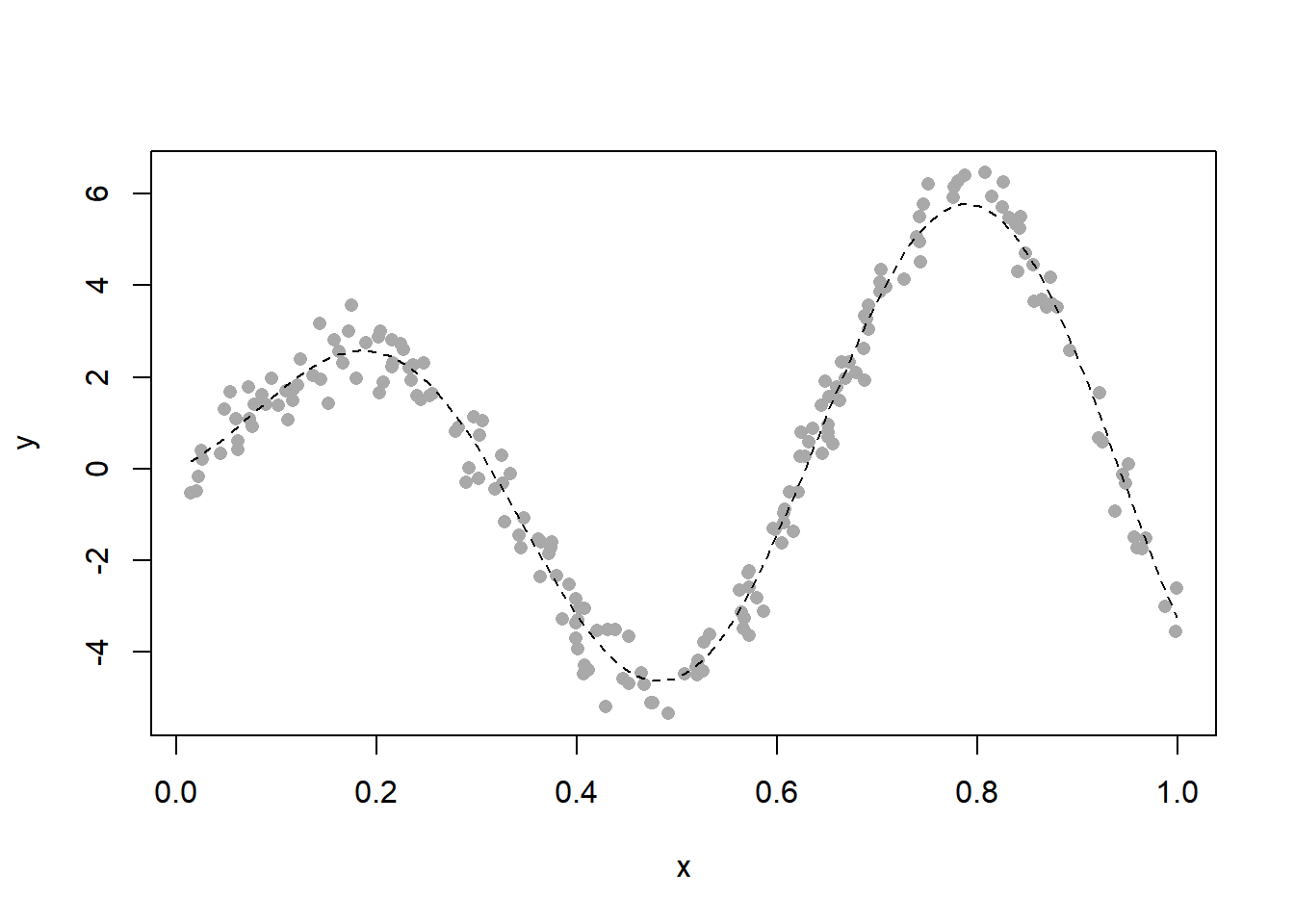

x_new = seq(0, 1, len = 1000) # for plotting purposes

21.1.1 Kernel smoothing

We use the Gaussian kernel (aka heat kernel).

plot(x, y, pch = 16, col = "darkgrey")
curve(f, lty = 2, add = TRUE)

h = 0.05 # bandwidth
fit = ksmooth(x, y, "normal", bandwidth = h, x.points = x_new)
lines(x_new, fit$y, col = "darkred", lwd = 2)

h = 0.15 # bandwidth
fit = ksmooth(x, y, "normal", bandwidth = h, x.points = x_new)
lines(x_new, fit$y, col = "darkgreen", lwd = 2)

h = 0.25 # bandwidth
fit = ksmooth(x, y, "normal", bandwidth = h, x.points = x_new)
lines(x_new, fit$y, col = "darkblue", lwd = 2)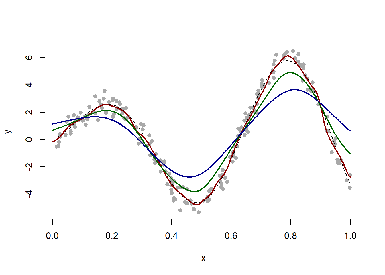

Notice how the last two estimators are grossly biased near \(x = 1\). ### Choice of bandwidth by cross-validation With a visual exploration, a choice of bandwidth around \(h = 0.05\) seems best. But we notice that the estimator is biased, particularly at the extremes and at the boundary. We use cross-validation to choose the bandwidth to optimize prediction. Monte Carlo leave-k-out cross-validation is particularly easy to implement.

h_grid = seq(0, 0.1, len = 20) # grid of bandwidth values
m = round(n/10) # size of test set
B = 1e2 # number of monte carlo replicates
pred_error = matrix(NA, 20, B) # stores the prediction error estimates
for (k in 1:20) {
  h = h_grid[k]
  for (b in 1:B) {
    test = sort(sample(1:n, m))
    fit = ksmooth(x[-test], y[-test], x.points = x[test], "normal", bandwidth = h)
    pred_error[k, b] = sum((fit$y - y[test])^2)
  }
}
pred_error = apply(pred_error, 1, mean)
plot(h_grid, pred_error, type = "b", pch = 15, lwd = 2, xlab = "bandwidth", ylab = "estimated prediction error")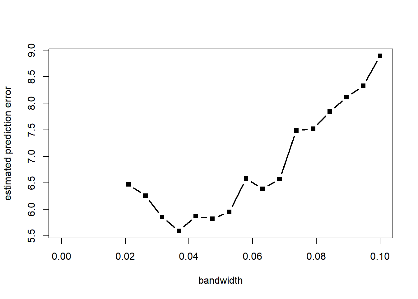

h = h_grid[which.min(pred_error)] # selected bandwidth
plot(x, y, pch = 16, col = "darkgrey")
curve(f, lty = 2, add = TRUE)
fit = ksmooth(x, y, "normal", bandwidth = h, x.points = x_new) # corresponding fit
lines(x_new, fit$y, col = "darkblue", lwd = 2)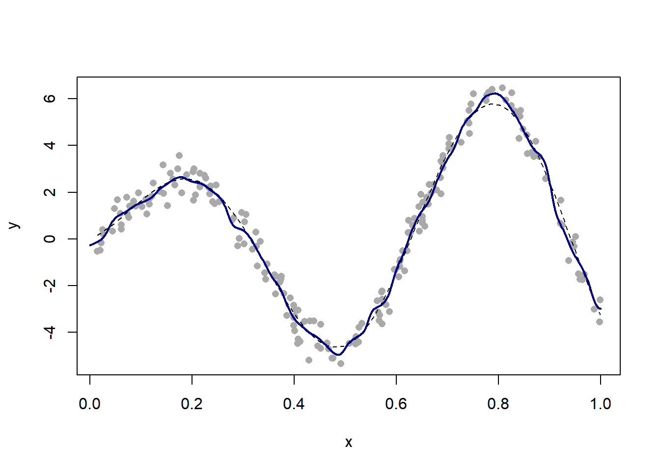

21.1.2 Local linear regression

(See the manual for explanation of what the parameter “span” stands for. It essentially controls the number of nearest neighbors.)

require(MASS)
plot(x, y, pch = 16, col = "darkgrey")
curve(f, lty = 2, add = TRUE)
fit = loess(y ~ x, span = 0.2)
val = predict(fit)
lines(x, val, col = "darkblue", lwd = 2)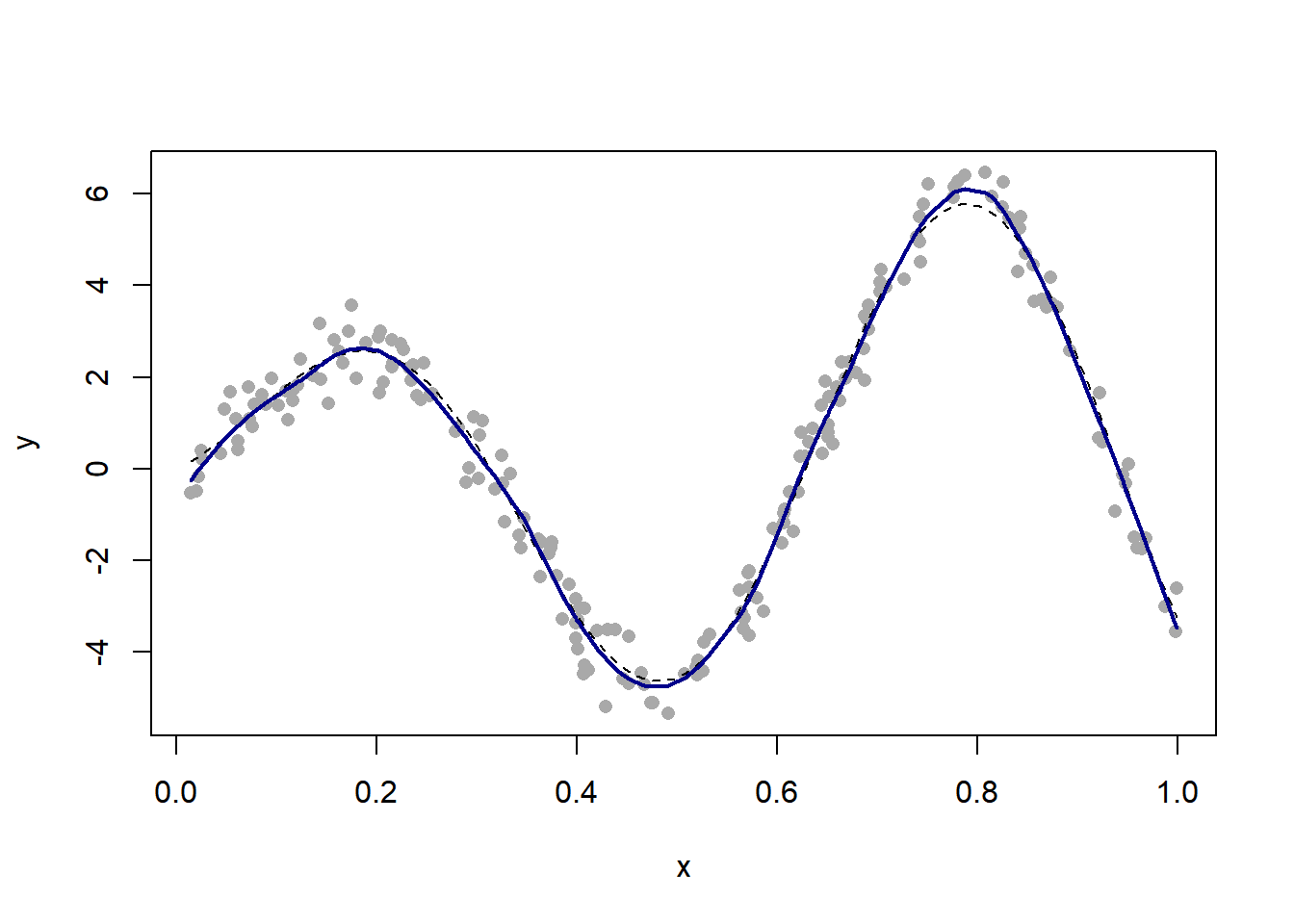

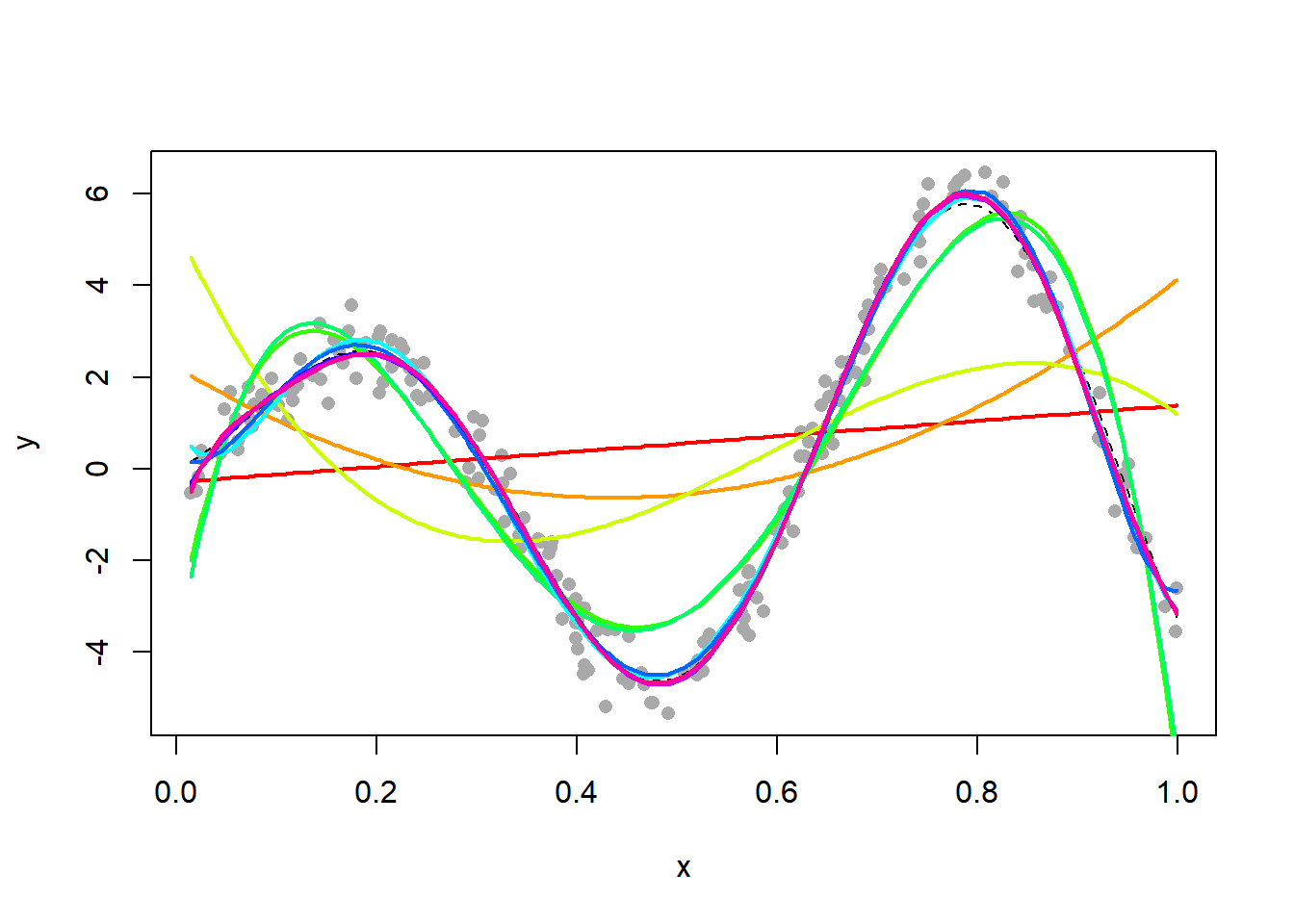
21.1.3 Polynomial regression

We now fit a polynomial of varying degree. This is done using the function, which fits linear models (and polynomial models are linear models)according to the least squares criterion.

plot(x, y, pch = 16, col = "darkgrey")
curve(f, lty = 2, add = TRUE)
for (d in 1:10) {
  fit = lm(y ~ poly(x, degree = d))
  lines(x, fit$fitted, lwd = 2, col = rainbow(10)[d])
}

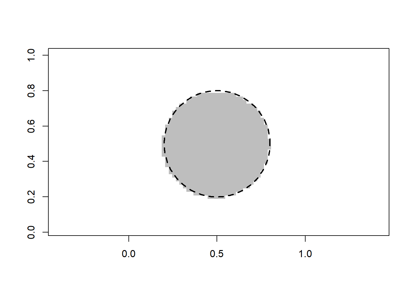
21.2 Classification

We consider the following synthetic dataset.

n = 2000 # sample size
x1 = runif(n) # first predictor variable
x2 = runif(n) # second predictor variable
x = cbind(x1, x2)
y = as.numeric((x1-0.5)^2 + (x2-0.5)^2 <= 0.09) # response variable (two classes)
plot(x1, x2, pch = 16, col = y+2, asp = 1, xlab = "", ylab = "")
rect(0, 0, 1, 1, lty = 3)
require(plotrix)
draw.circle(0.5, 0.5, 0.3, lty = 2, lwd = 2)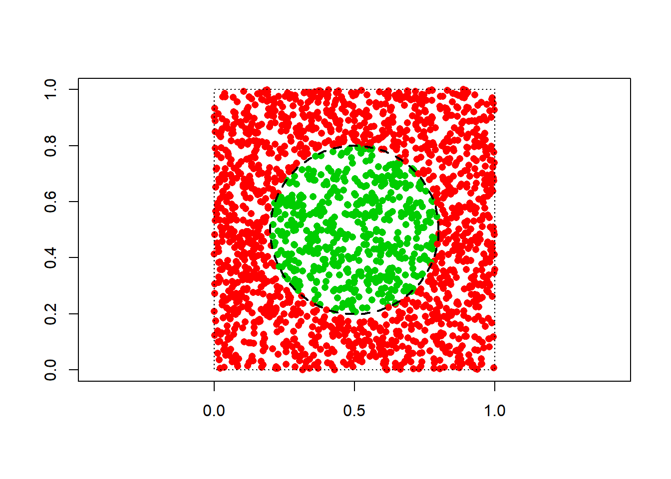

21.2.1 Nearest neighbor classifier

Nearest neighbor majority voting is readily available. (\(k\) below denotes the number of neighbors.)

require(class)
m = 50 
x_new = (1/m) * cbind(rep(1:m, m), gl(m, m)) # gridpoints
par(mfrow = c(2, 2))
class_color = c("white", "grey")
for (k in c(1, 3, 7, 10)) {
  val = knn(x, x_new, y, k = k)
  val = as.numeric(as.character(val))
  plot(x_new[, 1], x_new[, 2], pch = 15, col = class_color[val+1], asp = 1, xlab = "", ylab = "", main = paste("number of neighbors:", k))
  draw.circle(0.5, 0.5, 0.3, lty = 2, lwd = 2)
}

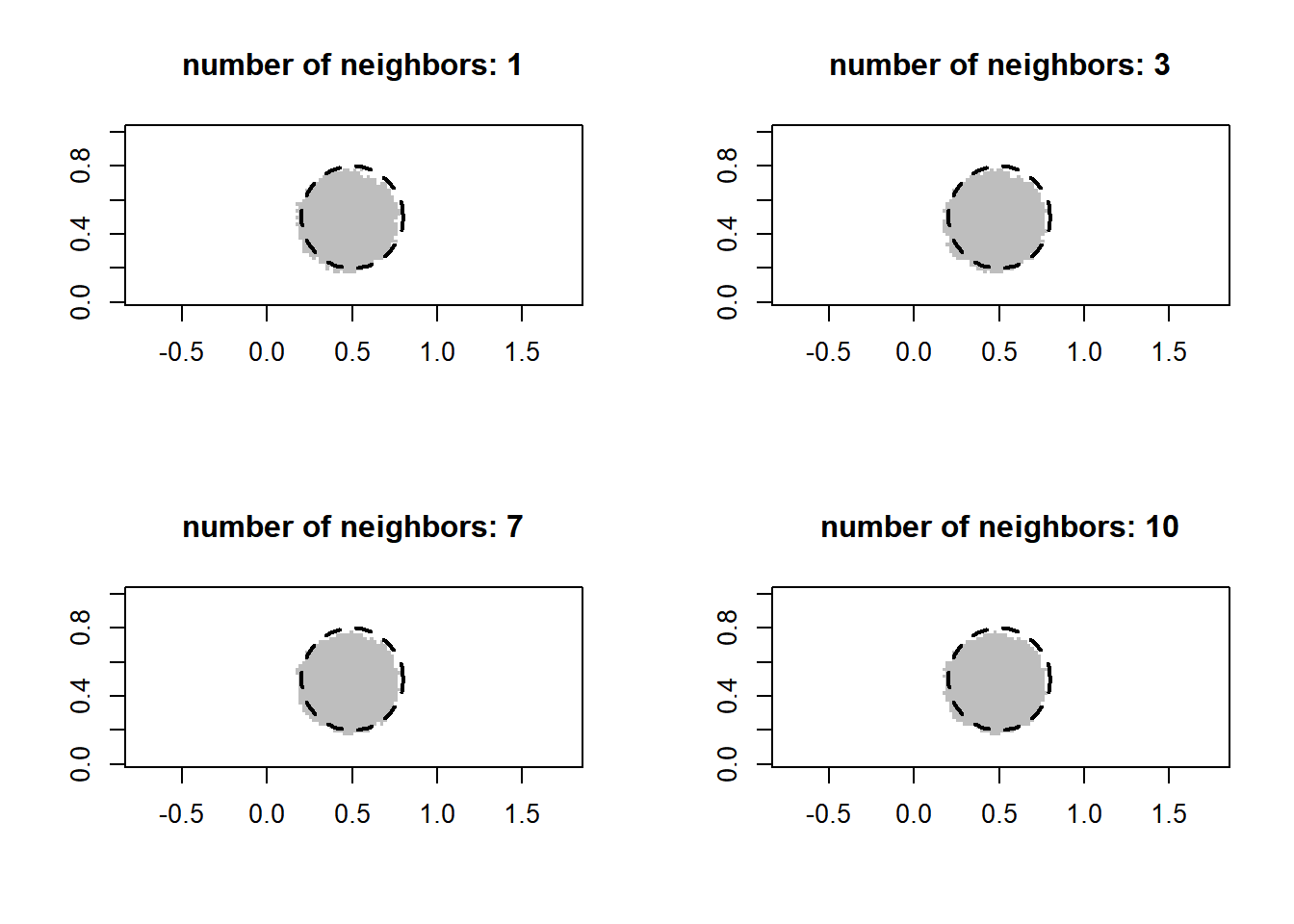
The classifier does not seem very sensitive to the choice of the number of nearest neighbors. Nevertheless, we can of course apply cross-validation to choose that parameter. The following implements leave-out-out cross-validation.

k_max = 30 # maximum number of neighbors
pred_error = numeric(k_max)
for (k in 1:k_max) {
  fit = knn.cv(x, y, k = k)
  pred_error[k] = sum(fit != y)
}
plot(1:k_max, pred_error, type = "b", pch = 15, lwd = 2, xlab = "number of neighbors", ylab = "estimated prediction error")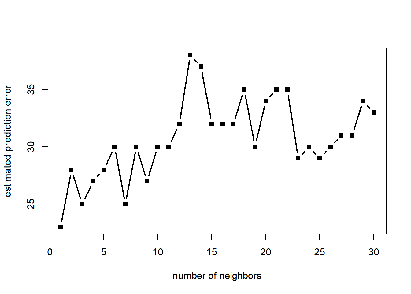

which.min(pred_error) 

[1] 1

The selected value of the parameters (number of neighbors) varies substantially from simulation to simulation, likely due to the fact that the sample size is relatively small. ### Linear classification We first apply logistic regression based on a polynomial of degree 2 in the predictor variable(s). The fit is excellent (as expected).

dat = data.frame(x1 = x[, 1], x2 = x[, 2], y = y)
x_new = data.frame(x1 = x_new[, 1], x2 = x_new[, 2])
fit = glm(y ~ x1 + x2 + x1*x2 + I(x1^2) + I(x2^2), data = dat, family = "binomial")
prob = predict(fit, x_new, type = "response") # estimated probabilities
val = round(prob) # estimated classes
plot(x_new[, 1], x_new[, 2], pch = 15, col = class_color[val+1], asp = 1, xlab = "", ylab = "")
draw.circle(0.5, 0.5, 0.3, lty = 2, lwd = 2)

We now turn to support vector machines (with a polynomial kernel of degree 2). The fit is excellent (as expected).

require(kernlab)
dat$y = as.factor(dat$y)
fit = ksvm(y ~ ., data = dat, kernel = "polydot", kpar = list(degree = 2))
val = predict(fit, x_new, type = "response")
val = as.numeric(as.character(val))
plot(x_new[, 1], x_new[, 2], pch = 15, col = class_color[val+1], asp = 1, xlab = "", ylab = "")
draw.circle(0.5, 0.5, 0.3, lty = 2, lwd = 2)