2 Discrete Probability Spaces

2.1 Bernoulli trials

Generating a sequence of Bernoulli trials of a given length and with a given probability parameter

n = 10 # length of the sequence
p = 0.5 # probability parameter
X = sample(c("H","T"), n, replace=TRUE, prob=c(p,1-p))

noquote(X)

 [1] H H H H H T H T H T

The number of heads in that sequence

sum(X == "H")

[1] 7

2.2 Sampling without replacement

An urn with \(r\) red ball and \(b\) blue balls represented as a vector

r = 7
b = 10
urn = c(rep("R", r), rep("B", b))
noquote(urn)

 [1] R R R R R R R B B B B B B B B B B

Sampling uniformly at random without replacement from that urn a given number of times

n = 5
X = sample(urn, n)
noquote(X)

[1] B R B B B

2.3 Pólya’s urn model

A direct (and naive) implementation of Pólya’s urn model

polyaUrn = function(n, r, b){
  # n: number of draws
  # r: number of red balls
  # b: number of blue balls
  urn = c(rep("R", r), rep("B", b))
  X = character(n) # stores the successive draws
  for (i in 1:n){
    draw = sample(urn, 1)
    X[i] = draw
    if (draw == "R"){
      urn = c("R", urn)
    } else {
      urn = c(urn, "B")
    }
  }
  return(X)
}

X = polyaUrn(10, 2, 3)
noquote(X)

 [1] R B R R R B R B R R

2.4 Factorials and binomials coefficients

Factorials are quickly very large. To see this, we plot the first few in logarithmic scale (in base 10).

n = 200
plot(0:n, log10(factorial(0:n)), type="l", lwd=2, ylab="factorials (log in base 10)", xlab="integers")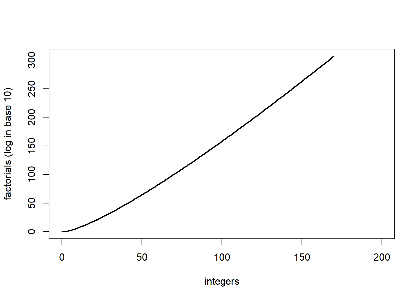

The factorials exceeds the maximum possible number in R, which is given by the following.

.Machine$double.xmax

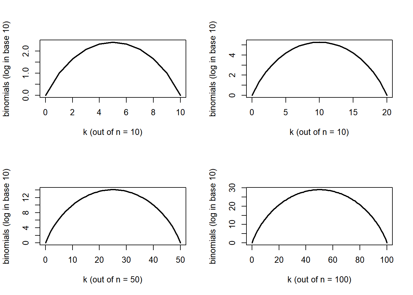
[1] 1.797693e+308

Binomials are also large numbers for the most part.

par(mfrow = c(2, 2))

n = 10
plot(0:n, log10(choose(n, 0:n)), type="l", lwd=2, ylab="binomials (log in base 10)", xlab="k (out of n = 10)")

n = 20
plot(0:n, log10(choose(n, 0:n)), type="l", lwd=2, ylab="binomials (log in base 10)", xlab="k (out of n = 10)")

n = 50
plot(0:n, log10(choose(n, 0:n)), type="l", lwd=2, ylab="binomials (log in base 10)", xlab="k (out of n = 50)")

n = 100
plot(0:n, log10(choose(n, 0:n)), type="l", lwd=2, ylab="binomials (log in base 10)", xlab="k (out of n = 100)")