3 Discrete Distributions

3.1 Uniform distributions

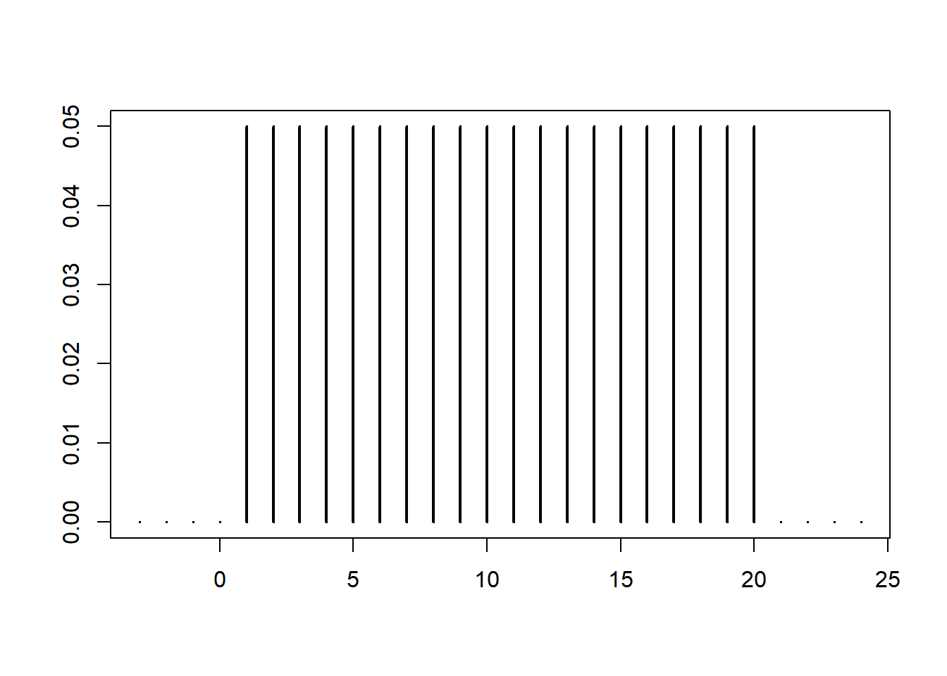
Consider the uniform distribution on \(\{1, \dots, n\}\).

n = 20

Its mass function (when defined on the integers) is given by

dunid = function(k, n) (1/n)*(1 <= k)*(k <= n)

Here is a graph of this function

k = -3:(n+4)
plot(k, dunid(k, n), type = "h", lwd = 2, xlab = "", ylab = "")

Its distribution function (when defined on the reals) is given by

punid = function(x, n) pmin(1, pmax(0, floor(x))/n)

Here is a graph of this function

curve(punid(x, n), 0, n, 1e3, lwd = 2, xlab = "", ylab = "")
abline(h = 0, lty = 2)
abline(h = 1, lty = 2)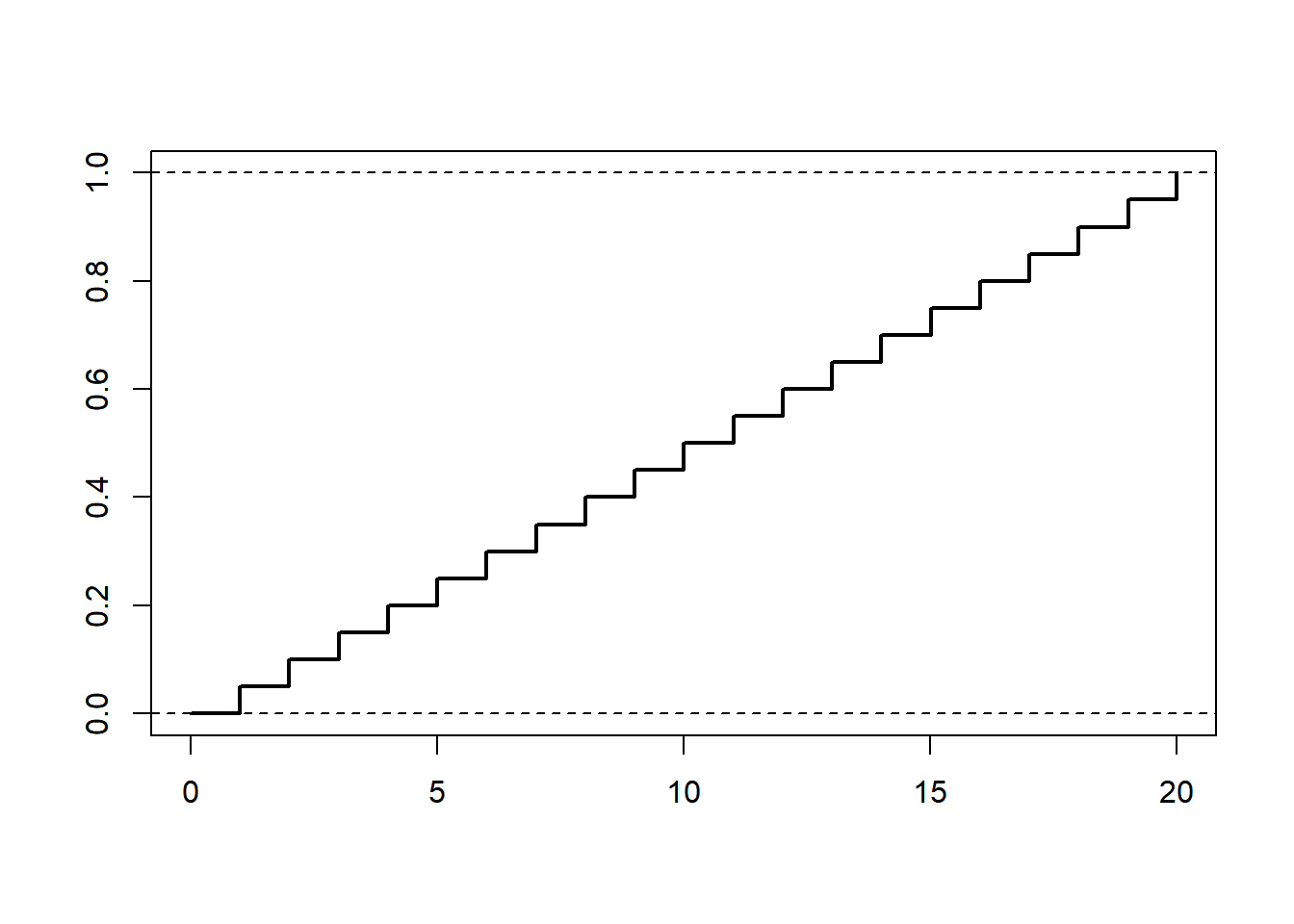

3.2 Binomial distributions

Consider the binomial distribution with the following parameters.

n = 20
p = 0.2

Here is a plot of its mass function

k = -3:(n+4)
plot(k, dbinom(k, n, p), type = "h", lwd = 2, xlab = "", ylab = "")

Here is a plot of its (cumulative) distribution function

curve(pbinom(x, n, p), -1, n, 1e3, lwd = 2, xlab = "", ylab = "")
abline(h = 0, lty = 2)
abline(h = 1, lty = 2)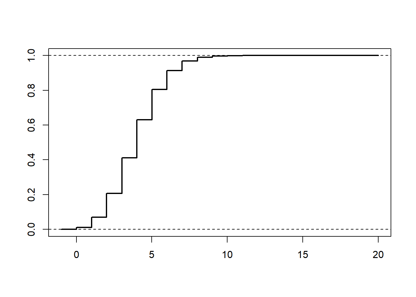

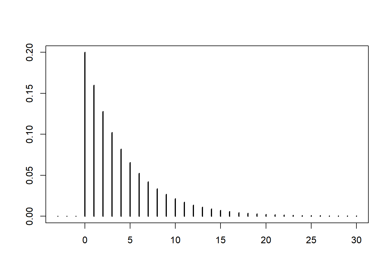
3.3 Geometric distributions

p = 0.2

Here is a plot of its mass function

k = -3:30
plot(k, dgeom(k, p), type = "h", lwd = 2, xlab = "", ylab = "")

Here is a plot of its (cumulative) distribution function

curve(pgeom(x, p), -1, 30, 1e3, lwd = 2, xlab = "", ylab = "")
abline(h = 0, lty = 2)
abline(h = 1, lty = 2)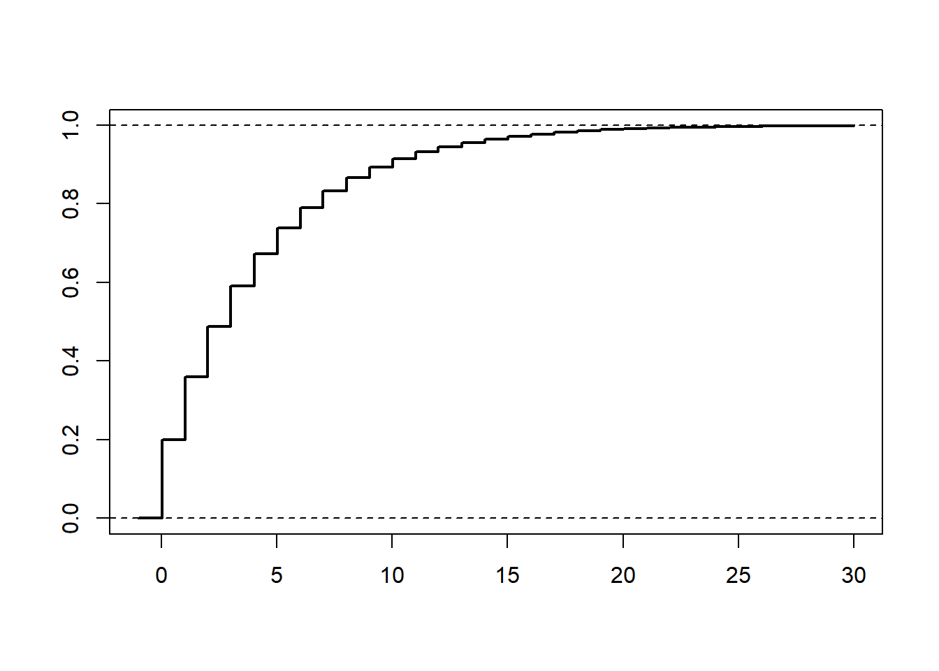

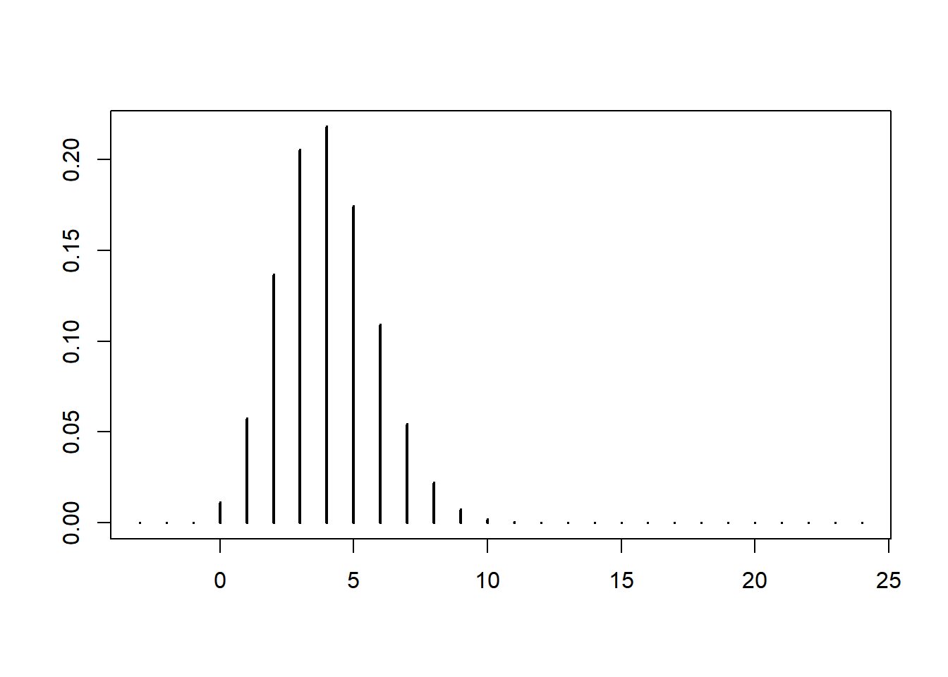
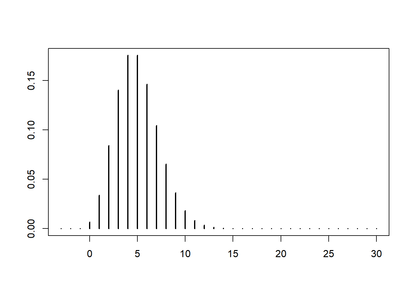
3.4 Poisson distributions

lambda = 5

Here is a plot of its mass function

k = -3:30
plot(k, dpois(k, lambda), type = "h", lwd = 2, xlab = "", ylab = "")

Here is a plot of its (cumulative) distribution function

curve(ppois(x, lambda), -1, 30, 1e3, lwd = 2, xlab = "", ylab = "")
abline(h = 0, lty = 2)
abline(h = 1, lty = 2)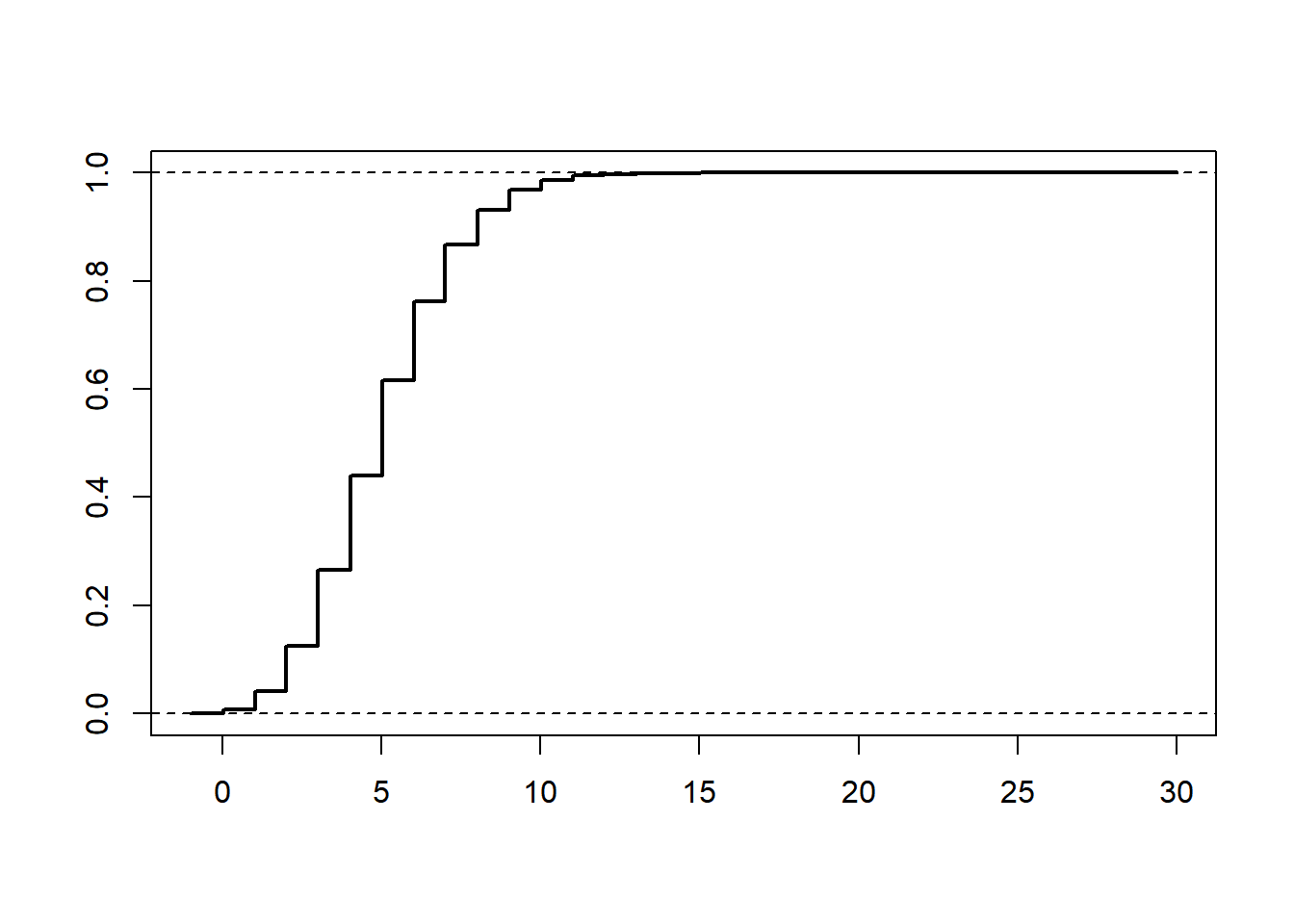

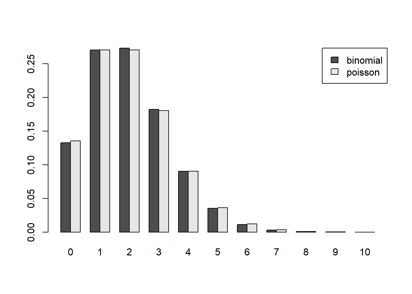
Let’s check the validity of the Law of Large Numbers.

n = 100
p = 2/n
lambda = n*p
k = 0:10
tab = rbind(dbinom(k, n, p), dpois(k, lambda))
rownames(tab) = c("binomial", "poisson")
colnames(tab) = k
barplot(tab, beside = TRUE, legend = TRUE, args.legend=list(x = "topright"), names.arg = k)