19 Correlation Analysis
We work with the famous dataset that Pearson collected on the heights of men and their sons. An appropriate plot is the scatterplot.
require(UsingR)
plot(father.son, pch = 16, xlab = "father's height", ylab = "son's height", asp = 1)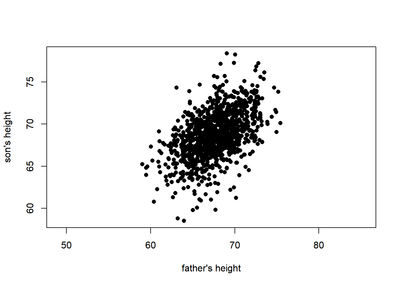
19.1 Sample correlations
We compute various types of correlations between the son and father heights.
[1] 0.5013383[1] 0.5058485[1] 0.349275319.2 Correlations tests
Although it is pretty clear from the scatterplot that the father and son heights are positively correlated (or more generally, monotonically associated), for pedagodical reasons, we perform the corresponding tests. (Look at the manual for details on how the p-values are computed. In the present case, the first and third are approximated based on asymptotic theory, while the second is based on exact calculations but the p-value is only approximated because of ties.)
    Pearson's product-moment correlation

data:  sheight and fheight
t = 19.006, df = 1076, p-value < 2.2e-16
alternative hypothesis: true correlation is not equal to 0
95 percent confidence interval:
 0.4552586 0.5447396
sample estimates:
      cor
0.5013383
    Spearman's rank correlation rho

data:  sheight and fheight
S = 103172697, p-value < 2.2e-16
alternative hypothesis: true rho is not equal to 0
sample estimates:
      rho
0.5058485
    Kendall's rank correlation tau

data:  sheight and fheight
z = 17.174, p-value < 2.2e-16
alternative hypothesis: true tau is not equal to 0
sample estimates:
      tau
0.3492753
19.3 Distance covariance (and test)
We also apply the distance covariance test. (The function returns the Monte Carlo permutation p-value based on R replicates.)
    dCov independence test (permutation test)

data:  index 1, replicates 1000
nV^2 = 742.04, p-value = 0.000999
sample estimates:
     dCov
0.8296702