10 Sampling and Simulation
10.1 Monte Carlo simulations
In the 5-card poker game, the probability of a flush is \(1/508 \approx 0.00197\). It’s a good exercise to derive this number analytically based on combinatorics. We can approximate this number using Monte Carlo simulations (based on the Law of Large Numbers) by simply repeatedly generating a poker hand and checking whether it’s a flush or not. Since the number we are estimating is quite small, the number of Monte Carlo replicates has to be quite large to result in a decent approximation. We use some code taken from a probability course at Duke University.
source("https://www2.stat.duke.edu/courses/Spring12/sta104.1/Homework/poker_simulation.R")
B = 1e5 # number of MC replicates
number_flush = 0
for (b in 1:B) {
  x = deal_hand()
  number_flush = number_flush + (what_hand(x) == "Flush")
}
cat(sprintf("fraction of flush hands (out of %i): %f", B, number_flush/B))
fraction of flush hands (out of 100000): 0.00207010.2 Monte Carlo integration
Simulations, again via the Law of Large Numbers, allow for the computation of integrals, since integrals can be interpreted as expectations. This avenue offers some advantages over numerical integration such as ease of implementation (although code for numerical integration is readily available) and lower computational complexity in higher dimensions (in fact as low as \(3\)). We perform some numerical experiments in dimension one where a Monte Carlo approach is typically less desirable, but where we can more easily quantify its accuracy as compared to numerical integration.
f = function(x){sqrt(x)}
exact_integral = 2/3 # integral over [0, 1]
num_integral = function() {
  integrate(f, 0, 1)$value
} # numerical integration
mc_integral = function() {
  x = runif(1e6)
  return(mean(f(x)))
} # MC integration with 1e6 replicates

# accuracy
num_error = num_integral() - exact_integral
num_error
[1] 7.483435e-08S = 1e2
mc_error = numeric(S)
for (s in 1:S) {
mc_error[s] = mc_integral() - exact_integral
}
summary(mc_error) Min. 1st Qu. Median Mean 3rd Qu. Max.
-8.196e-04 -1.283e-04 4.566e-05 3.157e-05 1.963e-04 6.626e-04 # speed
require(benchr)
summary(benchmark(num_integral(), mc_integral(), times = 100, progress = FALSE), digits = 3, row.names = FALSE)Time units : microseconds
expr n.eval min lw.qu median mean up.qu max total relative
num_integral() 100 22.8 25.8 29.9 54.6 75.1 452 5460 1
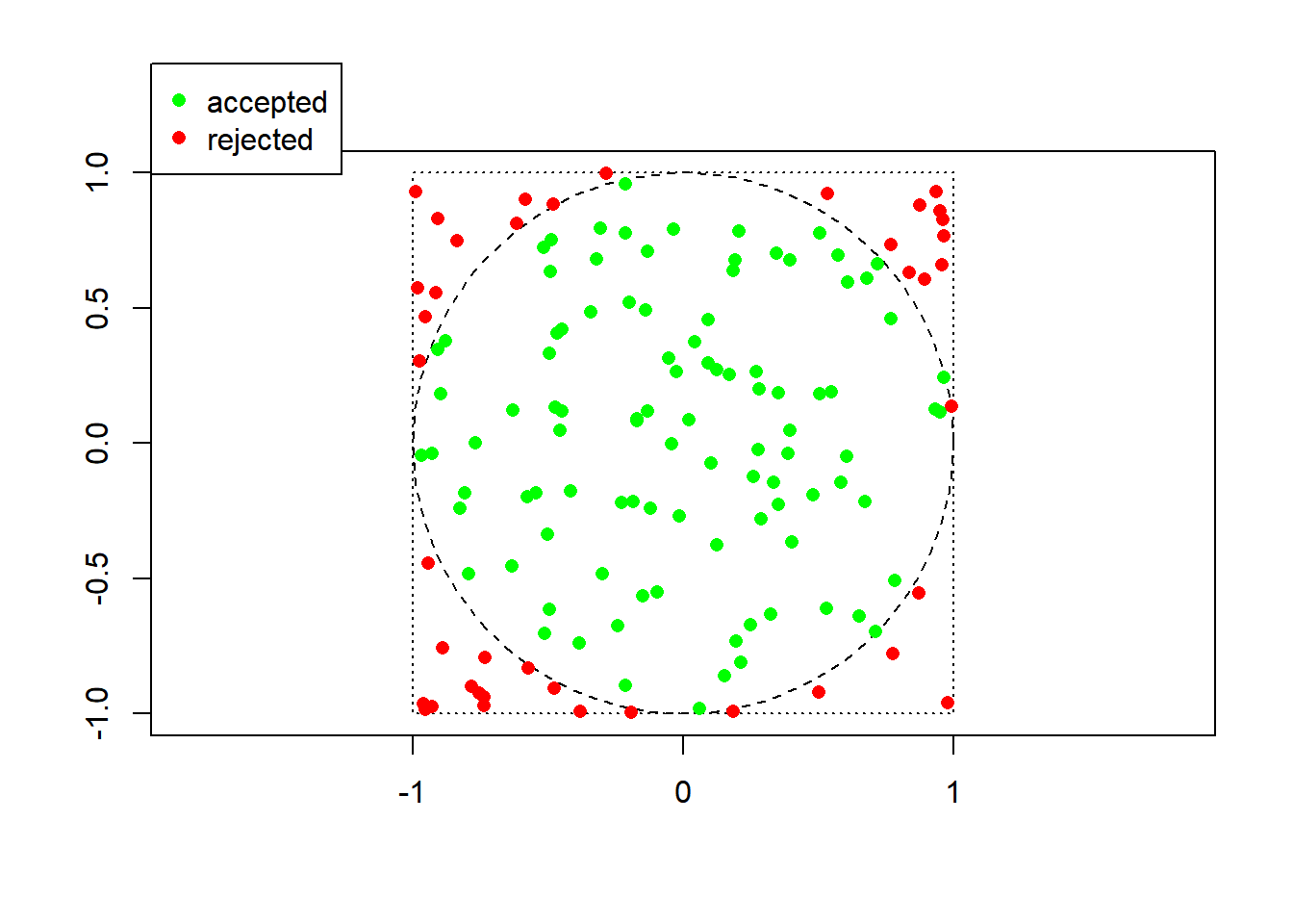
mc_integral() 100 31500.0 31900.0 33100.0 34700.0 36000.0 67300 3470000 1110In dimension one, at least for this simple function, numerical integration is much superior in both accuracy and speed, as expected. In higher dimensions, numerical integration may not even be feasible… ## Rejection sampling Here is a simple example of rejection sampling, where the goal is to sample uniformly at random from the unit disc. The approach is based on sampling the unit square (which contains the unit disc) uniformly at random (which is easy) and only keeping those draws that fall in the disc.
require(plotrix)
plot(0, 0, type = "n", xlim = c(-1,1), ylim = c(-1,1), xlab = "", ylab = "", asp = 1)
draw.circle(0, 0, 1, lty = 2)
rect(-1, -1, 1, 1, lty = 3)
legend("topleft", c("accepted", "rejected"), col = c("green", "red"), pch = 16, xpd = TRUE, inset = c(0, -0.15))

n = 100 # desired sample size
t = 0 # number of samples drawn from the proposal distribution
while (t < n) {
  y = runif(2, -1, 1)
  color = "red"
  if (y[1]^2 + y[2]^2 <= 1) {
    t = t+1
    color = "green"
  }
  points(y[1], y[2], pch = 16, col = color)
}
10.3 Markov chain Monte Carlo
For illustration, we consider the setting of species co-occurrence, important in Ecology, where a presence-absence matrix is available, and we want to draw uniformly at random from the set of binary matrices of same size and with the same row and column totals. This is one of the random models considered in that field, meant to represent a situation where the various species have populated the various geographical sites “at random”. The Markov chain consists in swapping \(2 \times 2\) submatrices whenever possible.
                         Seymour Baltra Isabella Fernandina Santiago Rabida Pinzon Santa.Cruz Santa.Fe San.Cristobal Espanola Floreana Genovesa Marchena Pinta Darwin Wolf
Geospiza magnirostris          0      0        1          1        1      1      1          1        1             1        0        1        1        1     1      1    1
Geospiza fortis                1      1        1          1        1      1      1          1        1             1        0        1        0        1     1      0    0
Geospiza fuliginosa            1      1        1          1        1      1      1          1        1             1        1        1        0        1     1      0    0
Geospiza difficilis            0      0        1          1        1      0      0          1        0             1        0        1        1        0     1      1    1
Geospiza scandens              1      1        1          0        1      1      1          1        1             1        0        1        0        1     1      0    0
Geospiza conirostris           0      0        0          0        0      0      0          0        0             0        1        0        1        0     0      0    0
Camarhynchus psittacula        0      0        1          1        1      1      1          1        1             0        0        1        0        1     1      0    0
Camarhynchus pauper            0      0        0          0        0      0      0          0        0             0        0        1        0        0     0      0    0
Camarhynchus parvulus          0      0        1          1        1      1      1          1        1             1        0        1        0        0     1      0    0
Platyspiza crassirostris       0      0        1          1        1      1      1          1        1             1        0        1        0        1     1      0    0
Cactospiza pallida             0      0        1          1        1      0      1          1        0             1        0        0        0        0     0      0    0
Cactospiza heliobates          0      0        1          1        0      0      0          0        0             0        0        0        0        0     0      0    0
Certhidea olivacea 1 1 1 1 1 1 1 1 1 1 1 1 1 1 1 1 10 0 1 1 1 1 1 1 1 1 0 1 1 1 1 1 1
1 1 1 1 1 1 1 1 1 1 0 1 0 1 1 0 0
1 1 1 1 1 1 1 1 1 1 1 1 0 1 1 0 0
0 0 1 1 1 0 0 1 0 1 0 1 1 0 1 1 1
1 1 1 0 1 1 1 1 1 1 0 1 0 1 1 0 0
0 0 0 0 0 0 0 0 0 0 1 0 1 0 0 0 0
0 0 1 1 1 1 1 1 1 0 0 1 0 1 1 0 0
0 0 0 0 0 0 0 0 0 0 0 1 0 0 0 0 0
0 0 1 1 1 1 1 1 1 1 0 1 0 0 1 0 0
0 0 1 1 1 1 1 1 1 1 0 1 0 1 1 0 0
0 0 1 1 1 0 1 1 0 1 0 0 0 0 0 0 0
0 0 1 1 0 0 0 0 0 0 0 0 0 0 0 0 0
1 1 1 1 1 1 1 1 1 1 1 1 1 1 1 1 1B = 1e4 # number of steps in the Markov chain
I = diag(2)
J = matrix(c(0, 1, 1, 0), 2, 2)
X = as.matrix(finches)
rownames(X) = NULL
colnames(X) = NULL
for (b in 1:B) {
rows = sample(1:nrow(X), 2)
cols = sample(1:ncol(X), 2)
if (sum(X[rows, cols] == I) == 4) X[rows, cols] = J
if (sum(X[rows, cols] == J) == 4) X[rows, cols] = I
}
write.table(X, row = FALSE, col = FALSE)1 0 1 1 1 1 1 1 1 1 1 1 1 1 1 0 0
1 1 1 1 1 0 1 1 1 1 0 1 0 1 1 1 0
1 0 1 1 1 0 1 1 1 1 1 1 1 1 1 0 1
0 0 1 1 1 1 1 1 1 1 0 1 0 0 1 0 0
0 1 1 1 1 1 1 1 0 1 0 1 1 1 1 0 0
0 0 0 1 1 0 0 0 0 0 0 0 0 0 0 0 0
0 0 1 1 0 1 1 1 1 0 0 1 0 1 1 1 0
0 0 1 0 0 0 0 0 0 0 0 0 0 0 0 0 0
0 0 1 1 1 1 1 1 1 1 0 1 0 0 1 0 0
0 1 1 1 1 1 1 0 1 1 0 0 0 1 1 0 1
0 0 1 0 1 1 0 1 0 1 0 1 0 0 0 0 0
0 0 0 0 0 0 0 1 0 0 0 1 0 0 0 0 0
1 1 1 1 1 1 1 1 1 1 1 1 1 1 1 1 1This code produces only {} approximately uniform random binary matrix (among those with the same row and column totals).