6 Multivariate Distributions
6.1 Multinomial distribution
We can draw from a multinomial distribution as follows
m = 5 # number of distinct values
p = 1:m
p = p/sum(p) # a distribution on {1, ..., 5}
n = 20 # number of trials
out = rmultinom(3, n, p) # each column is a realization of the corresponding multinomial distribution
rownames(out) = 1:m
colnames(out) = paste("Run", 1:3, sep = "")
out
Run1 Run2 Run3
1 3 1 1
2 1 2 1
3 3 5 8
4 3 6 4
5 10 6 6We can evaluate the probability of a particular draw
[1] 0.004355026.2 Uniform distributions
Here is the density of the uniform distribution on the unit square \([0,1]^2\).
dunif2 = function(x, y){
  (0 <= x)*(x <= 1)*(0 <= y)*(y <= 1)
}
x = seq(-1, 2, len = 100)
y = seq(-1, 2, len = 100)
z = outer(x, y, dunif2)
persp(x, y, z, theta = 30, phi = 30, expand = 0.5, col = "lightblue", ltheta = 120, shade = 0.15, ticktype = "detailed")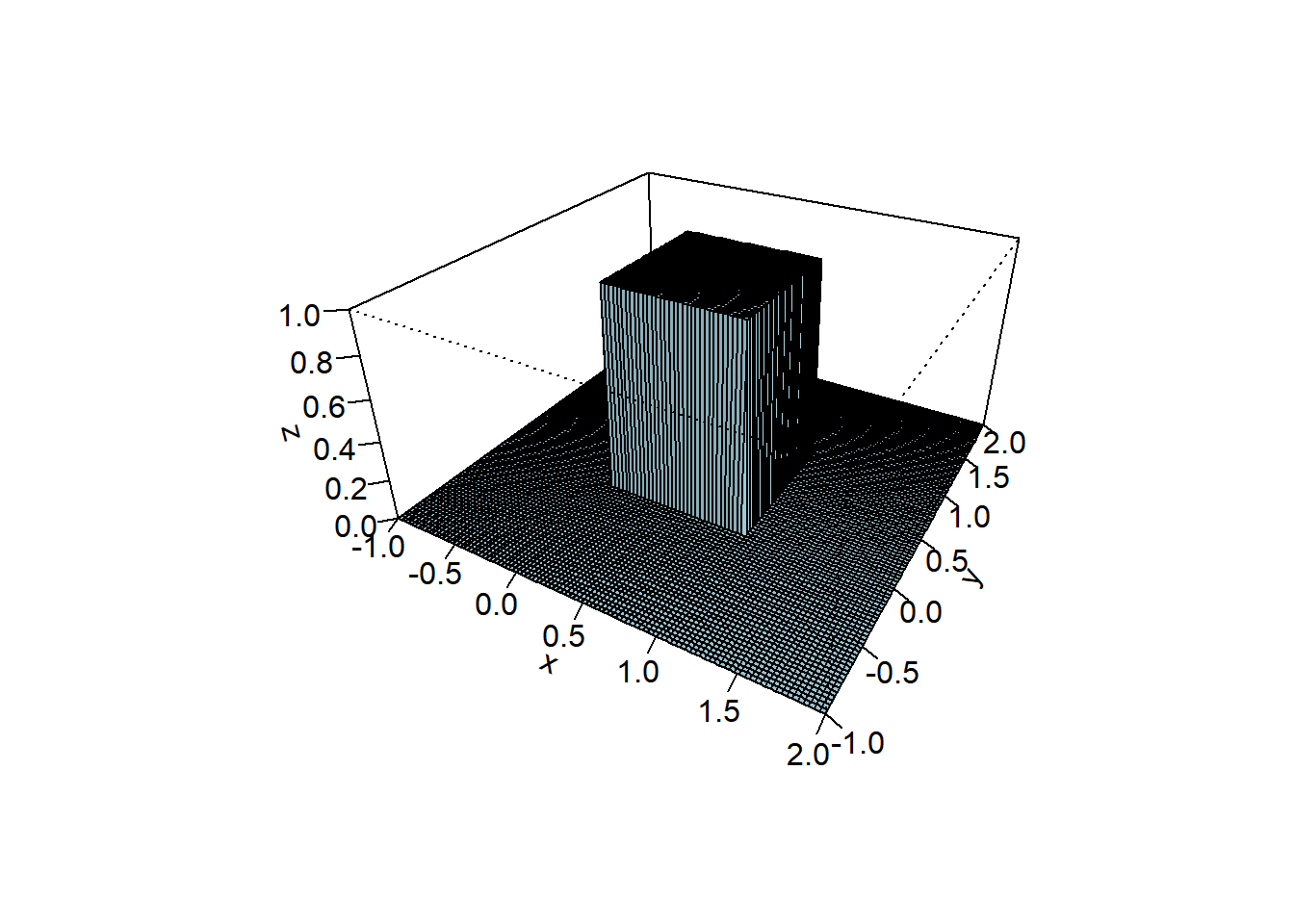
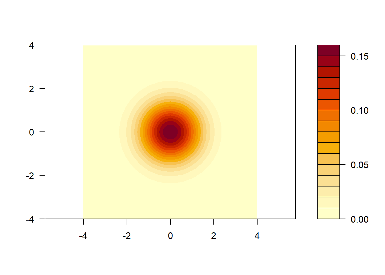
6.3 Normal distributions
Here is the density of the standard normal distribution (perspective plot and contour plot).
dnorm2 = function(x, y, mu = rep(0, 2), Sigma = diag(2)){
  v = as.vector(c(x, y) - mu)
  w = (2*pi*sqrt(det(Sigma)))^{-1} * exp(-(1/2) * t(v) %*% solve(Sigma) %*% v)
  as.vector(w)
}
require(mvtnorm)
dnorm2 = function(x, y, mu = rep(0, 2), Sigma = diag(2)){
  dmvnorm(cbind(x, y), mean = mu, sigma = Sigma)
}
x = seq(-4, 4, len = 100)
y = seq(-4, 4, len = 100)
z = outer(x, y, dnorm2)
persp(x, y, z, theta = 30, phi = 30, expand = 0.5, col = "lightblue", ltheta = 120, shade = 0.15, ticktype = "detailed")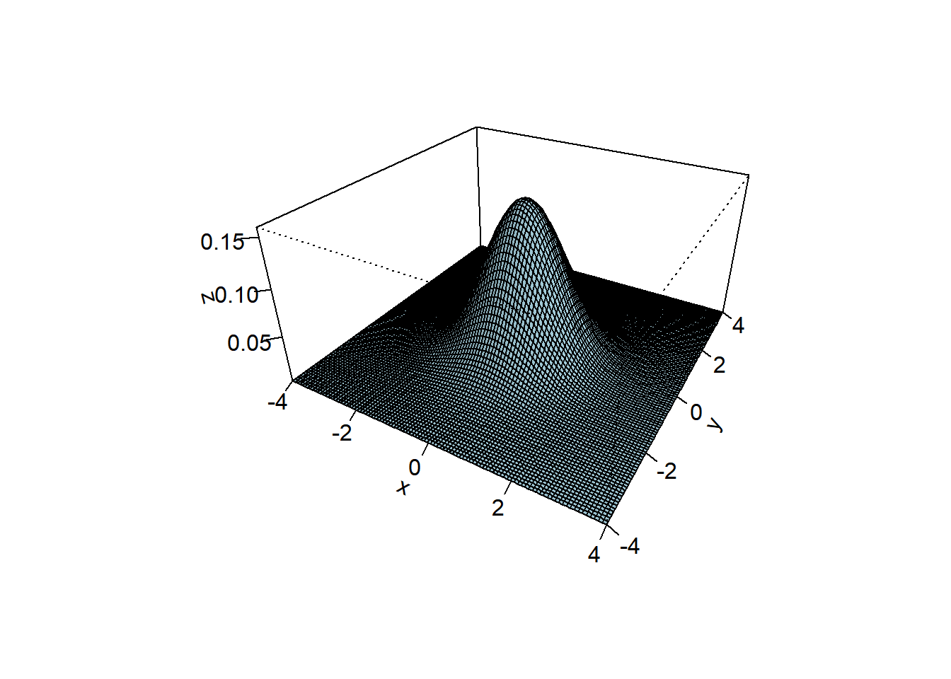
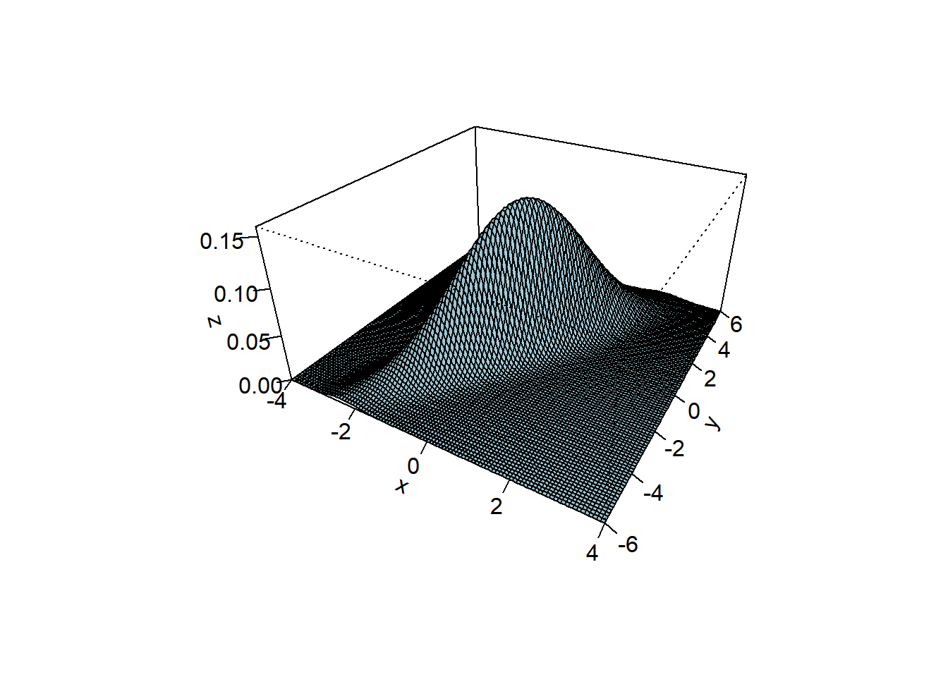
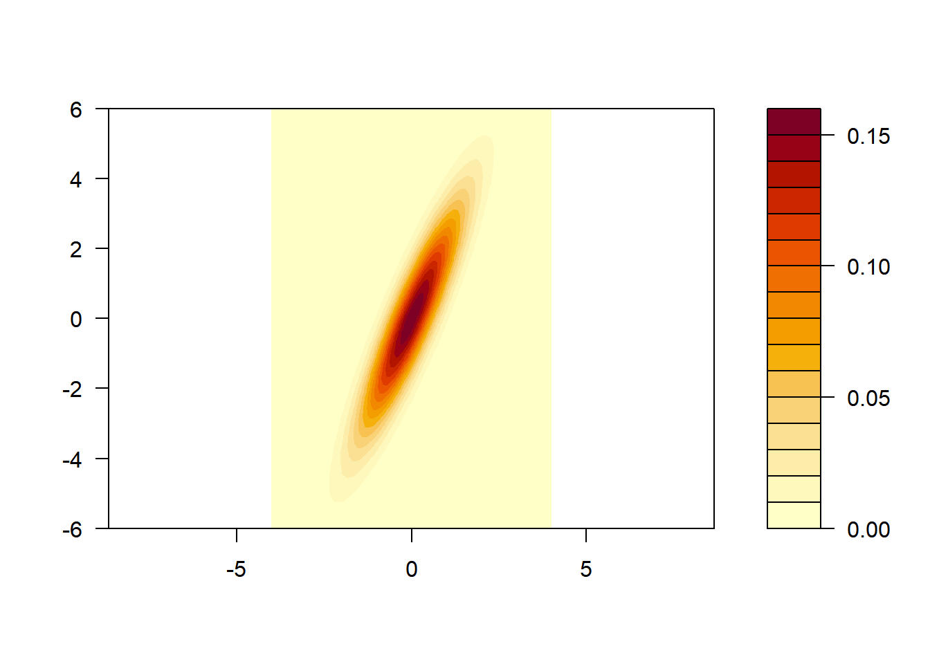
And here is the density of the normal distribution with mean zero and covariance matrix \(\begin{pmatrix}1 & 2 \\ 2 & 5\end{pmatrix}\).
M = matrix(c(1, 2, 2, 5), 2, 2)
x = seq(-4, 4, len = 100)
y = seq(-6, 6, len = 100)
z = outer(x, y, dnorm2, Sigma = M)
persp(x, y, z, theta = 30, phi = 30, expand = 0.5, col = "lightblue", ltheta = 120, shade = 0.15, ticktype = "detailed")