8 Convergence of Random Variables
8.1 Law of Large Numbers
We illustrate the theorem in the context of a sequence of iid Bernoulli random variables. We fix the parameter at \(p = 0.3\). We then consider a varying number \(n\) of such random variables and the corresponding sums. We know that these are binomial with parameters \((n, p)\). The plot below draws, for each \(n\), the 10-percentile and the 90-percentile of \(\text{Bin}(n, p)\).
p = 0.3
n = 20*(1:50)
L = qbinom(0.10, n, p)/n
U = qbinom(0.90, n, p)/n
plot(n, rep(p, length(n)), type = "n", ylim = c(min(L), max(U)), xlab="n", ylab = "")
segments(n, L, n, U, lwd = 2, col = "black")
abline(h = p, lty = 2)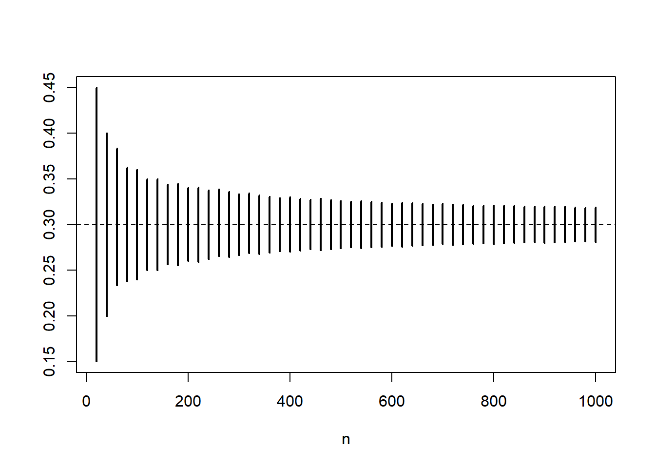
The convergence rate is so slow that the plot gives the impression that there is no convergence (in probability) to zero. To better see the convergence, we use a logarithmic scale.
n = 2^(10:20)
L = qbinom(0.10, n, p)/n
U = qbinom(0.90, n, p)/n
plot(n, rep(p, length(n)), log = "x", type = "n", ylim = c(min(L), max(U)), xlab="n", ylab = "")
segments(n, L, n, U, lwd = 2, col = "black")
abline(h = p, lty = 2)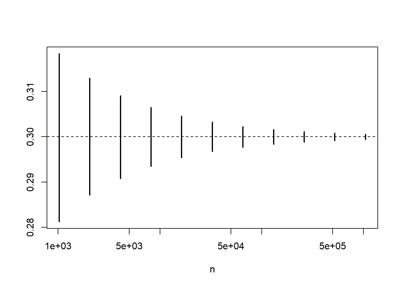
The plots above illustrate the Law of Large Numbers in terms of convergence in probability, i.e., in its weak version. The strong version asserts that the convergence is in fact with probability one, when we look at entire realizations of sequences of partial means.
We start by looking at a few realizations of such mean sequences.
B = 10 # number of trial sequences
N = 1e2 # trial sequence length
trials = matrix(rbinom(B*N, 1, p), B, N) # each row represents a trial sequence
partial_sums = apply(trials, 1, cumsum) # each column is a partial sum sequence
partial_means = partial_sums/N # each column is a partial mean sequence
matplot(partial_means, type = "l", lty = 1, col = rainbow(B), xlab = "n", ylab = "")
abline(h = p, lty = 2)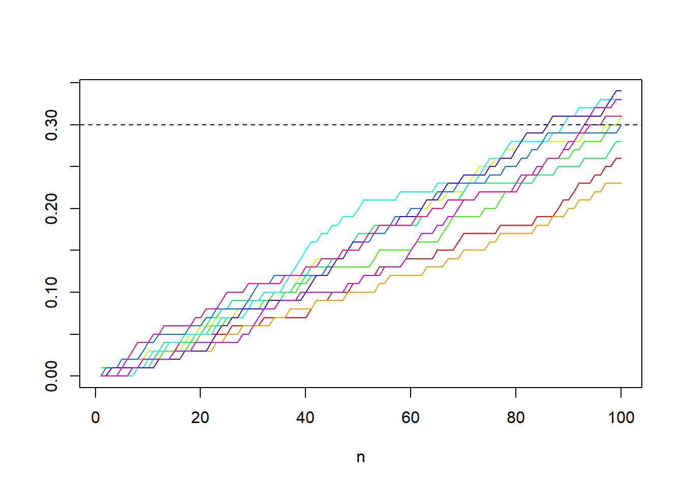
We now generate many such mean sequences and plot them.
B = 1e2 # number of trial sequences
N = 1e4 # trial sequence length
trials = matrix(rbinom(B*N, 1, p), B, N) # each row represents a trial sequence
partial_sums = apply(trials, 1, cumsum) # each column is a partial sum sequence
partial_means = partial_sums/N # each column is a partial mean sequence
matplot(partial_means, type = "l", lty = 1, col = "grey", xlab = "n", ylab = "")
abline(h = p, lty = 2)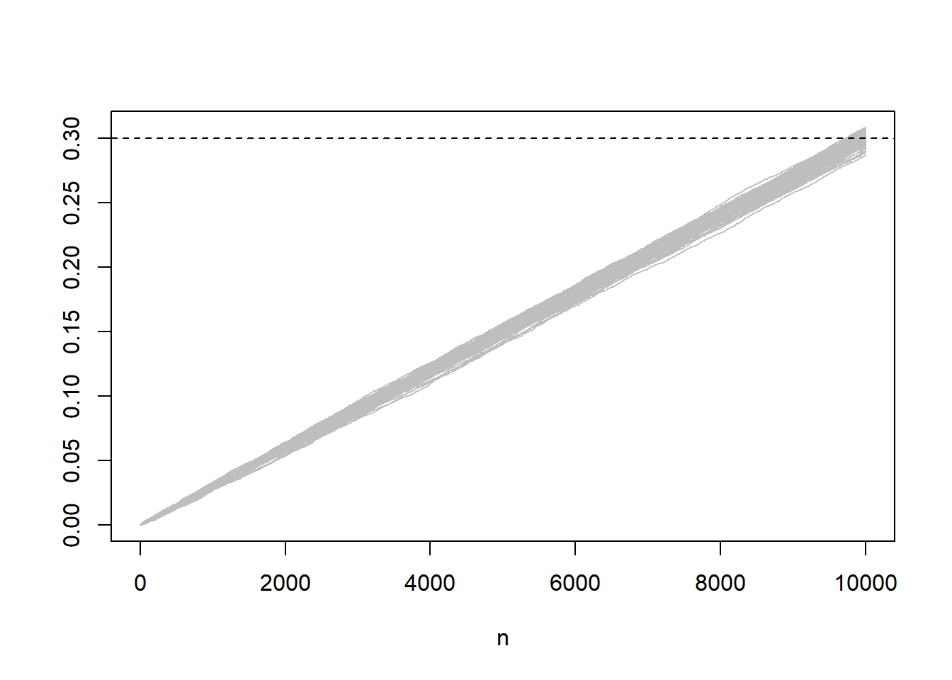
8.2 Central Limit Theorem
The Law of Large Numbers provides a first-order limit, which is deterministic: The sequence of partial means converges to the mean of the underlying distribution generating the random variables. The Central Limit Theorem provides a second-order limit, which does not exists in a deterministic sence, but does in the distributional sense: The sequence of partial means, when standardized, converges in distribution to the standard normal distribution. (This assumes that the underlying distribution has finite second moment.)
To see this, we go back to the first setting above, but we track down multiple quantiles of the successive (standardized) binomial distributions.
p = 0.3
n = 20*(1:50)
Q = matrix(NA, 50, 9) # each row stores the quantiles of standardized binomial distribution
for (k in 1:50){
  Q[k, ] = (qbinom((1:9)/10, n[k], p) - n[k]*p)/sqrt(n[k]*p*(1-p))
}
matplot(n, Q, type = "l", lty = 1, lwd = 2, col = 4, xlab = "n", ylab = "quantiles")
abline(h = qnorm((1:9)/10), lty = 2) # quantiles of the standard normal distribution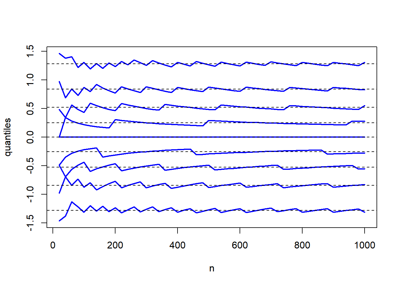
If instead of tracking down the distributions of the standardized sums, we track down actual realizations of the standardized sums (i.e., standardized random walks), we observe that there is (again) no deterministic convergence. There is a way in which a limit can be defined, and it turns out to be a stochastic process known as Brownian motion. However, given that a regular computer can only deal with discrete objects, a Brownian motion is typically generated as such a standardized sum, so the result is in a sense difficult to illustrate. We content ourselves with simply showing a single realization.
N = 1e4
trials = rbinom(N, 1, p)
partial_sums = cumsum(trials)
standardized_partial_sums = (partial_sums - (1:N)*p)/sqrt((1:N)*p*(1-p))
plot(1:N, standardized_partial_sums, type = "l", lwd = 2, xlab = "n", ylab = "")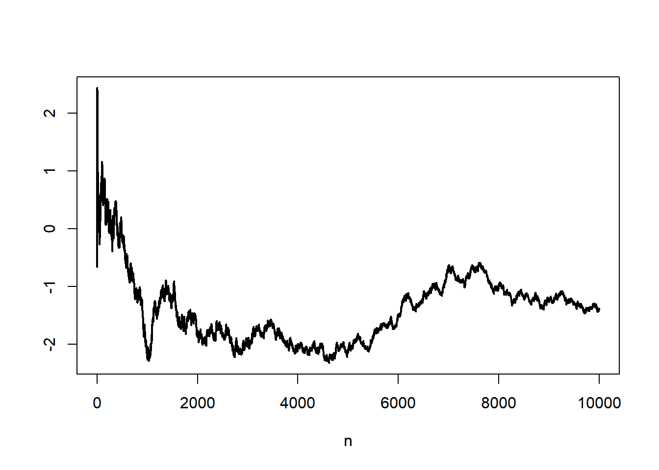
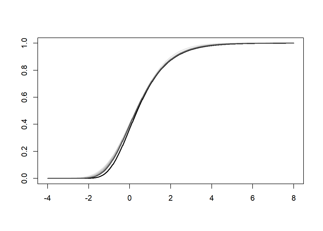
8.3 Extreme Value Theory
Let us consider the setting of a normal sample and let us look at the maximum. The Extreme Value Theorem applies and says that this maximum will converge, when properly standardized, to a Gumbel distribution (and the proper standardization can be worked out).
n = c(1e1, 1e2, 1e3, 1e4, 1e5)
# normalization sequences
a = sqrt(2*log(n))
b = - 2*log(n) + (1/2)*log(log(n)) + (1/2)*log(4*pi)
# plot of the Gumbel distribution
z = seq(-4, 8, len  = 1e3)
plot(z, exp(-exp(-z)), lwd = 2, type = "l", xlab = "", ylab = "")
# plot of the distribution of each standardized maximum (one of each sample size)
max_cdf = matrix(NA, length(z), length(n))
for (k in 1:length(n)){
  max_cdf[, k] = pnorm((z - b[k])/a[k])^n[k]
}
matlines(z, max_cdf, lty = 1, lwd = 2, col = grey.colors(length(n), rev = TRUE))