7 Expectation and Concentration

7.1 Concentration inequalities

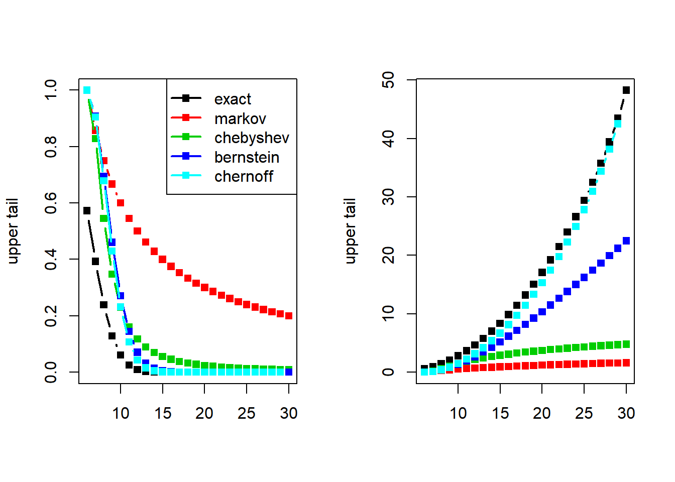
Let us compare the accuracy of some of the main concentration inequalities for the binomial distribution. We consider \(Y\) binomial with parameters \((n, p)\) specified below, and compute the bounds given by Markov, Chebyshev, Bernstein, and Chernoff.

n = 30
p = 0.2
mu = n*p # mean
sigma = sqrt(n*p*(1-p)) # standard deviation
y = ceiling(mu):n

Exact upper tail:

exact = pbinom(y-1, n, p, lower.tail = FALSE)

Markov’s upper bound:

markov = mu/y

Chebyshev’s upper bound:

chebyshev = 1/(1 + (y-mu)^2/sigma^2)

Bernstein’s upper bound:

bernstein = exp(- ((y-mu)^2/2)/(sigma^2 + (y-mu)/3))

Chernoff’s upper bound:

b = y/n
chernoff = exp(- n*(b*log(b/p) + (1-b)*log((1-b)/(1-p))))

par(mfrow = c(1, 2))
matplot(y, cbind(exact, markov, chebyshev, bernstein, chernoff), type = "b", lty = 1, lwd = 2, pch = 15, xlab = "", ylab = "upper tail")
legend("topright", legend = c("exact", "markov", "chebyshev", "bernstein", "chernoff"), , lty = 1, lwd = 2, pch = 15, col = 1:5)
matplot(y, -log(cbind(exact, markov, chebyshev, bernstein, chernoff)), type = "b", lty = 1, lwd = 2, pch = 15, xlab = "", ylab = "upper tail") # applying a log transformation to zoom in on the tails