16 One Numerical Sample
The following dataset was published in the paper “Measurement of Treadware of Commercial Tires” published in Rubber Age in 1953. Each tire was subject to tread wear measurements by two methods, the first based on weight loss (WGT) and the second based on groove wear (GRO). Importantly, these measurements are paired by tire. We take the logarithm of the ratio.
16.1 Quantiles and other summary statistics
    Min.  1st Qu.   Median     Mean  3rd Qu.     Max.
-0.41985 -0.25247 -0.17578 -0.17229 -0.06516 0.02421 [1] -0.41985385 0.02421426 0% 20% 40% 60% 80% 100%
-0.41985385 -0.25593337 -0.18713311 -0.17278632 -0.06082956 0.02421426 [1] -0.175781[1] 0.08949068[1] -0.1722861[1] 0.1182363The boxplot is based on the extremes and the quartiles. (In this particular version, no points are labeled as outliers. This is not the default behavior.)
boxplot(wear, range = Inf, horizontal = TRUE, col = "grey", xlab = "tire wear (log ratio)")
rug(wear, lwd = 2) # adds a mark at each data points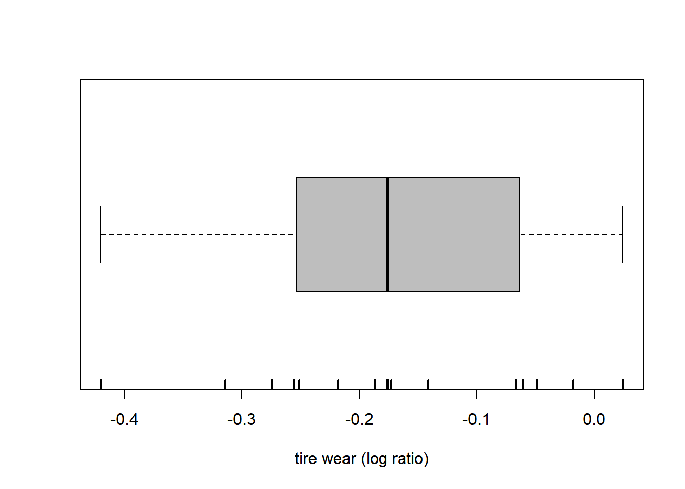
16.2 Empirical distribution function
Fun = ecdf(wear) # empirical distribution function
plot(Fun, lwd = 2, xlab = "tire wear (log ratio)", ylab = "cumulative probability", main = "Empirical distribution function")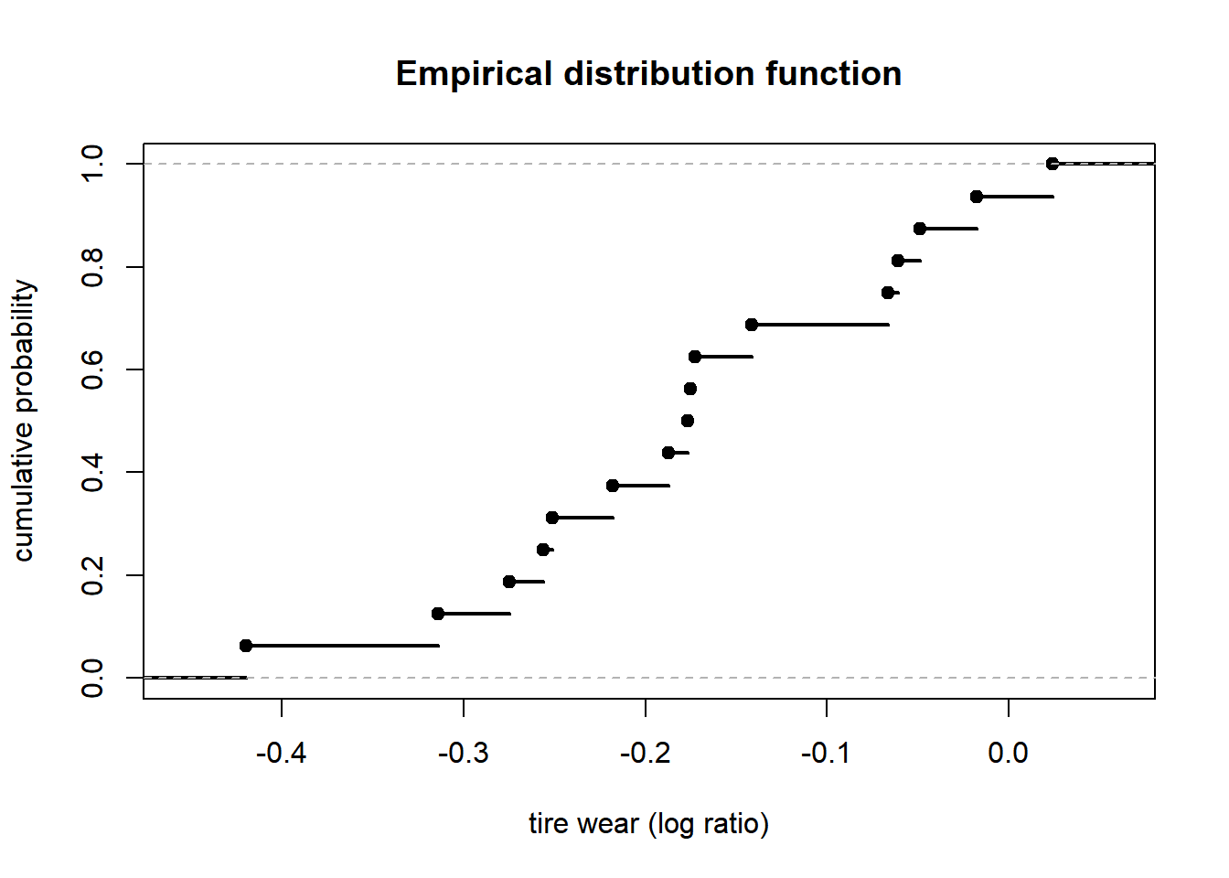
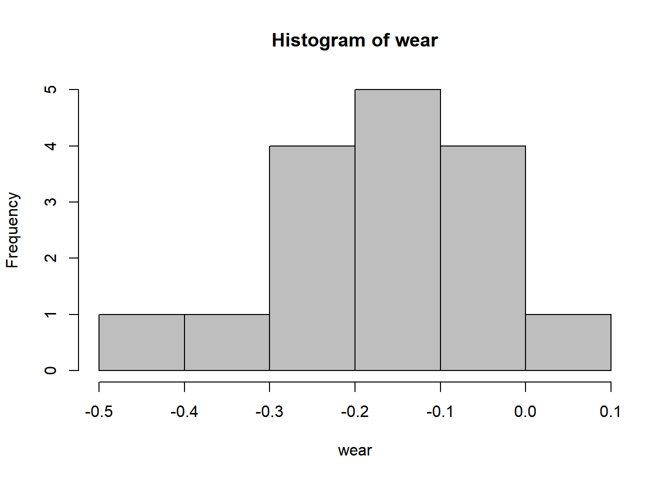
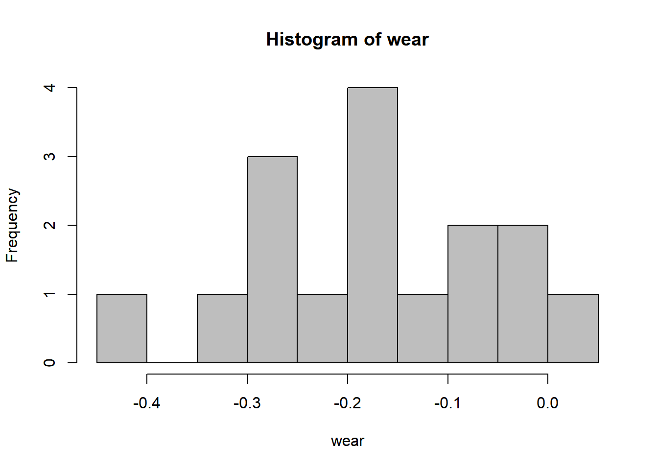
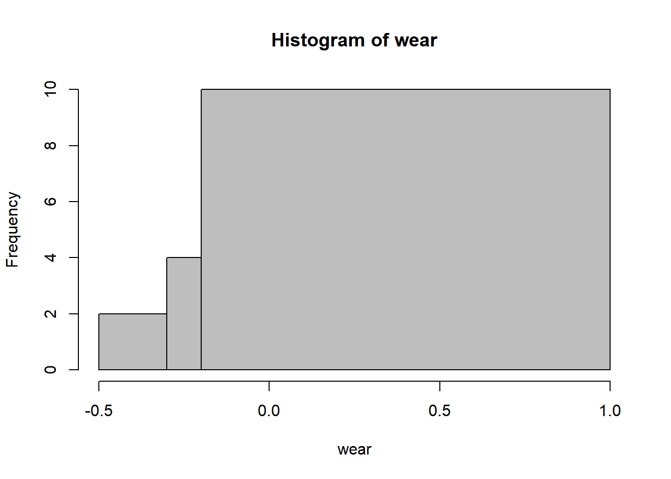
16.3 Histogram
16.4 Bootstrap confidence interval
We now look at a famous dataset collected by Pearson on the heights of adult men and their sons. This time we simply take the difference.
require(UsingR)
data(father.son)
height = with(father.son, sheight - fheight)
summary(height) # sons weight on average almost 1 inch more than their fathers!
Min. 1st Qu. Median Mean 3rd Qu. Max.
-8.9556 -0.8515 0.9629 0.9970 2.7484 11.2369 This is a larger dataset, allowing for a more sophisticated analysis. In particular, it is reasonable to compute a bootstrap confidence interval for the mean. Although it appears as easy to implement this by hand, we make a point of using a package. We compute the simplest interval, the percentile bootstrap confidence interval. (Note that the level is approximate, as usual with bootstrap confidence intervals.)
require(bootstrap)
B = 1e4 # number of bootstrap replicates
mean_boot = bootstrap(height, B, mean)
mean_boot = mean_boot[[1]] # bootstrapped means
alpha = 0.10 # desired confidence level is 1 - alpha
int = 2*mean(height) - quantile(mean_boot, c(1-alpha/2, alpha/2))
result = paste("bootstrap percentile", 1-alpha, "confidence interval: [", int[1], ",", int[2], "]")
cat(result)
bootstrap percentile 0.9 confidence interval: [ 0.857773691558442 , 1.13548268970315 ]16.5 Goodness-of-fit testing
For a more complex task, consider testing whether the data was generated from a normal distribution. To illustrate the situation we draw a histogram with the best fitting normal distribution (i.e., with parameters fitted by the method of moments) superimposed. The fit is very good.
hist(height, breaks = 50, freq = FALSE, col = "grey", xlab = "difference in height", main = "")
curve(dnorm(x, mean(height), sd(height)), min(height), max(height), add = TRUE, lty = 2, lwd = 2)
More formally, we apply the Lilliefors test, which confirms that the fit is good.
    Lilliefors (Kolmogorov-Smirnov) normality test

data:  height
D = 0.021301, p-value = 0.2767
Instead of a histogram, we can visualize the sample density using a kernel density estimate.
hist(height, breaks = 50, freq = FALSE, col = "grey", xlab = "difference in height", main = "")
lines(density(height), lwd = 2)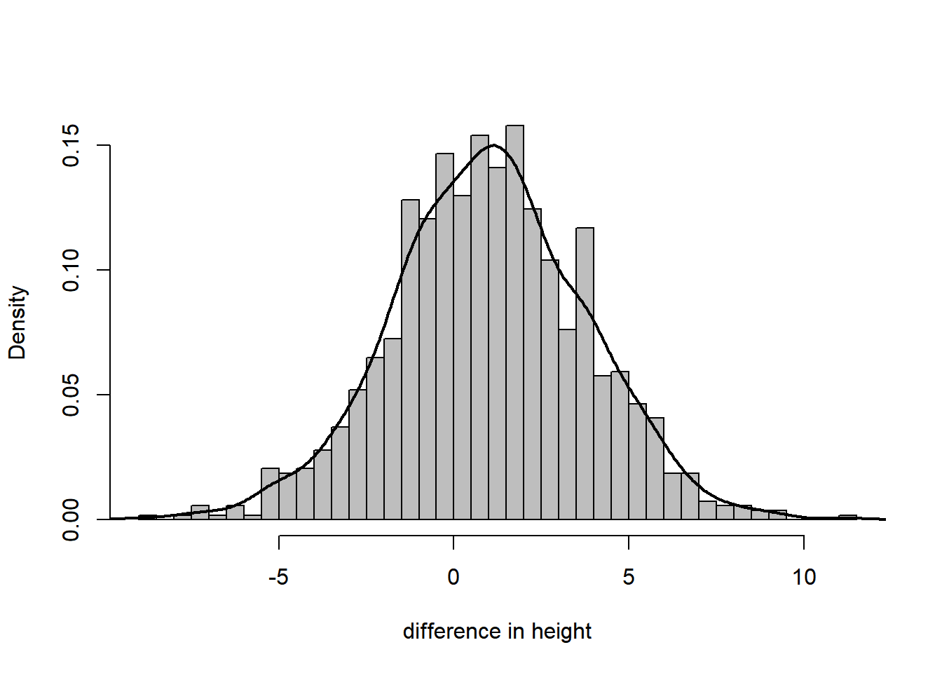
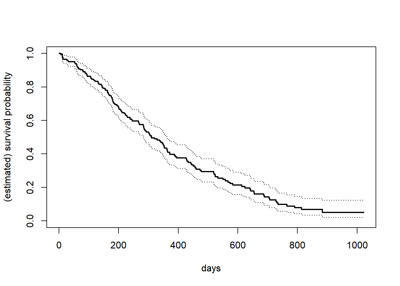
16.6 Kaplan–Meier estimator
Censored data is commonplace in survival analysis. We use the following specialized package, and the lung cancer dataset within it.
require(survival)
data(lung)
fit = survfit(Surv(time, status) ~ 1, data = lung) # Kaplan--Meier curve
plot(fit, xlab = "days", ylab = "(estimated) survival probability", lwd = c(2, 1, 1), lty = c(1, 3, 3))