Introduction to MATLAB

Welcome to the MATLAB component of Math 20D! If you are reading this, you have probably successfully logged in to a PC; if not, go here for instruction on how to do that. You now need to run both MATLAB and a word processor—we'll assume you're using Microsoft Word/ google docs. Instructions for that are here.

In the header of your Word document, be sure to include your name and PID.

As you complete a lab assignment, you should read along, enter all the commands listed in the tutorials, and work through the Examples. However, in your Word/google doc, you need only include your responses to the Exercises. Each response should clearly indicate which exercise it answers. The exercises will require different kinds of responses; the type of answer we are looking for will be marked by some combination of the icons described below.

Icon	Item	Comments
	Commands entered in MATLAB & resulting output	You should copy relevant input and output from MATLAB and paste it into your document. You need only include commands that worked. Screenshots are OK!
	Plots & graphs	Include all graphs generated in an exercise unless the problem specifically tells you which/how many to include. Screenshots are ok!
	Full sentence response	Answer questions with at least one or two complete sentences. Even if you're stuck, write down any reasoning or ideas you've had.
	Requires manual work	Do scratch work without using MATLAB. Record this work in your Word document, either by typing it or scanning it.

It is good practice to save your work as you go, in case of computer crash, power outage, etc.

We encourage you to talk to your fellow students while you work through the assignments. If you're stuck, try introducing yourself to your neighbor. Feel free to discuss responses to difficult exercises. However, in the end, you must submit your own work written in your own words!

Identical responses will be penalized at the grader's discretion!

Finally, there is one last important thing you should be aware of: the MATLAB quiz. Information about the quiz is available on the main page. Go back there and read that information now. Then complete this preliminary exercise. (This exercise will not be graded)

1. What is the date of your MATLAB quiz? What day of the week is that?
2. Where is your MATLAB quiz?

First Steps

Let's get started. After you've run MATLAB, it should be sitting there with a prompt:

When working through examples or exercises, you should omit the prompt (>>) and just type the commands that follow it (which are displayed like this). When you are given commands in either examples or exercises, instead of typing them into MATLAB yourself, you may want to consider copying the text from the webpage and pasting it into MATLAB next to the prompt. This can help avoid inadvertent errors.

Basic Operations

We can use MATLAB to do simple addition (+), subtraction (-), multiplication (*), division (/), and exponentiation (^).

ans =
   968

By far the most common source of errors in this course will be data entry errors—that is, errors made by typing commands or data incorrectly. Make sure you understand how MATLAB works with the order of operations, and use parentheses as needed to designate the correct order of operations. This will save you a lot of trouble down the road.

Elementary Functions

MATLAB includes many of the usual trigonometric and logarithmic functions, such as sin, cos, and log.

In MATLAB, log is not the base-10 logarithm log₁₀(x); rather, it's the natural logarithm log_e(x), which you've seen written as ln(x). We'll often also want to use the exponential function e^x. In MATLAB, we do not write this function as e^x. Instead, we use the built-in command exp. If we wanted to compute e^2, then, we would type exp(2).

Recall the formula for conversion of logarithms: log_b(x) = ^ln(x)⁄_ln(b). Use MATLAB and this formula to compute log₄(50). Include the input and output in your Word document.

Naming Variables

MATLAB allows us to use letters (or more generally, a letter followed by any string of letters, numbers, and underscores) to assign names to variables. This allows us to easily reuse past results.

>> a = sin(pi/12)

a =
   0.2588
   
>> b = cos(pi/12)

b =
   0.9659
   
>> result = a^2 + b^2

result =
   1

You can see here that pi is pre-assigned a value very close to π. In fact, MATLAB knows π to extreme accuracy, which we can see using the command vpa.

This command tells MATLAB to display the first argument (here, pi) to the chosen number of digits.

We saw in the last section that e is not pre-assigned. If we want e to have its usual value, we can assign it manually:

Hints & Tips

MATLAB has a number of time-saving features that are worth learning now.

The semicolon. Some commands in MATLAB will generate extremely long output. For example, try typing the following:

By examining the output, explain what the previous command did. (You need not include the output in your Word document.) How do you think MATLAB would respond if you typed m(26)? Try it.

On the other hand, if we enter the following: (notice the semicolon!)

there is no output. MATLAB has carried out the command, but the semicolon tells it not to print the result. If at some point later on, we'd like to see the output, we can do so by typing

For this course, we will usually include the semicolon in the example code if the output is excessively long or if the output is routine (for example, if we are just assigning a name to a constant and we already know what the output is going to be). Except in these two cases, you need to include any outputs related to the exercises.

Shift+Enter. We haven't had any need to do this so far, but it will be useful later to be able to run multiple inputs all at once, without typing out and running each line in sequence. You can jump to a new line without running your code by typing Shift+Return or Shift+Enter.

The up-arrow key. Bring up the main MATLAB window and try pushing the up-arrow key on the keyboard once. Then push it a few more times. Notice that this is bringing your previously-entered commands back onto the command line. You can also use the left and right arrow keys to position the cursor in a command in order to edit it. This is a great way to correct a command that had an error in it.

Suppose we want to evaluate the expression

Enter the command

>> z = 25-(100-7exp(5+cos(pi/3))

You will get an error message. Use the up-arrow to bring this line back, and then use the left and right arrow keys to correct the error(s). Include the wrong command, the error message, and your fix in your homework. [Hint: Multiplication and parentheses are good things to check.]

MATLAB's Built-in Help

While these labs are written to be as self-contained as possible, you may find that you've forgotten what a MATLAB command does, or you may wonder what else MATLAB can do. Fortunately, MATLAB has an extensive built-in help system. If you ever get stuck or need more info, one excellent way to get help in MATLAB is by entering

This command will take you to MATLAB's searchable documentation, where you can learn how to use all the built-in MATLAB commands by reading their help files. This is a particularly good resource when you know what you want to do but don't know which commands to use. For example, if you want to integrate something but don't know how, a search for "integral" will suggest both integral and int.

If you already know which command you want, but you've forgotten how exactly it works, one quick way to access its documentation is to enter help followed by the name of your command. This will usually give you a brief description of the command, some examples, and a list of related commands.

Compute arcsin(3) using MATLAB. Include the outputs in MATLAB. [Hint: Start by looking at help sin, or perhaps doc arcsine.]

If you are ever looking to get help with more general math topics, Wikipedia is an excellent resource.

For Loops & M-Files

If you haven't used MATLAB extensively before, at this point it may seem to be simply a powerful calculator. However, MATLAB has many features that will allow us to easily perform computations that would be very difficult or even impossible with a calculator. In this section we will look at two such tools: for loops and M-files.

For Loops

We often wish to perform a task repeatedly. MATLAB (along with most programming languages, for that matter) has a built-in tool known as a for loop. Suppose, for instance, that we wanted to print out the squares of the integers from 1 to 4. One option would be to type each square in individually. However, a better way to do a repetitive task like this is to use a for loop.

>> for i = 1:4
i^2
end

ans =
   1
ans =
   4
ans =
   9
ans =
   16

M-Files

As some problems get more complicated, or when they simply take a lot of commands to run, the command prompt window in MATLAB can become cumbersome. A better approach in such situations is to create and use an M-File. An M-file is a simple text file containing MATLAB commands that you can call from the regular MATLAB command window. M-Files can be either functions or chains of commands called scripts. We will mainly use them to define our own functions.

To create a new M-File, navigate to the top-left corner of the main MATLAB window and select on New Script. (Some versions of MATLAB may require you to select New ❯ Script or File ❯ New ❯ Blank M-File.) A text editor will appear, allowing you to enter the contents of the M-File and save it.

1    function printSquares
2    for i=1:4
3        i^2
4    end

Why is this useful? Well, for one thing, we don't need to retype the code for the loop every time we want to run it. We should be very thankful for this, since MATLAB programs can be quite long! For more complicated code, there are other reasons to use M-Files as well. Let's look at expanding the M-File above to make it more useful.

The M-File above prints the first four squares. But what if we wanted it to print the first 10? Well, one option would be to change the number in our M-File, save it, and then run it again at the prompt. However, there is an even better way to do it: we can allow the call to the M-File to accept as input the number of squares to print. Go back to your M-File and change it so that it now reads:

1    function printSquares(numberOfSquares)
2    for i=1:numberOfSquares
3        i^2
4    end

Be sure to save it again as "printSquares.m". Now run it at the command window by typing:

Try entering this command with values other than 10. As you can see, our code now prints out the first n squares, where n is the value you give as the argument for the printSquares function.

While MATLAB has a lot of built-in commands, it can't possibly have everything we would want built into it. Thus, M-Files are extremely important: they allow us to create our own MATLAB commands. Note that M-Files aren't limited to for loops, nor are they limited to just one input. The possibilities are endless.

We will look at one more example of the use of M-Files and for loops, but before we do, you'll create your own.

1. Recall that a geometric sequence is a sequence of the form a, ar, ar², ar³, …. At the MATLAB command prompt (not in an M-File), create a for loop that prints the first seven terms of this sequence when r=¹⁄₃ and a=1. Include the output in your Word document.
2. Create a new M-File named "geomSeq" with the loop above. Be sure to test it to make sure it works! Include the code for your M-File in your Word document.
3. Modify your M-File so that it accepts the value of r as an argument. Use this to find the first seven terms of the geometric sequence when r=1/4. Include the code that defines the function geomSeq in your Word document. Include also the output and the code you used in the command window.

Computing Series with For Loops

Recall that a geometric series is a series of the form a + ax + ax² + ax³, …. Geometric series appear in many applications, including compiling interest on bank accounts.

1    function sum = bal(yearlyDeposit,interestRate,years)
2    sum = 0;
3    for i=1:years
4        sum = sum + yearlyDeposit*(1+interestRate)^i;
5    end

ans =
   430.9136

There are a few differences between this loop and the ones above. The first major difference is that the first line now includes a variable, sum, followed by an equals sign, between the word function and the name of the M-File. This is telling the M-File to return the value of sum once the function has finished running. We also included semicolons to supress output of the loop, since now we are only interested in the final value and not the intermediate values. Removing semicolons can often be useful to see exactly what the function is doing, however; this is especially useful for finding bugs in a program.

The other thing to notice is that we have used a common programming trick for computing a series. In the first line of the function body we define the variable sum, which we set to zero initially. After each run of the loop, we compute the next term in the series and add that to sum. You can see this in line four, where we set sum equal to itself plus another term. This doesn't make much sense as a literal mathematical statement, but it's a common feature in programming languages. MATLAB reads this line and understands that it should update the value of sum by taking the old value and adding a new term. Thus each time our loop runs, it adds the new value to sum, and we keep a running total. This is a much more common use of for loops than printing out values. Let's have you give it a try with this next exercise.

1. Consider the series 1 + ¹⁄_r + ¹⁄_r² + ¹⁄_r³ + … + ¹⁄_rⁿ. Implement a calculation for this series in a new M-file, calling the function "mysum". The function should take two inputs, r and n. Copy the code from your new M-file into your document.
2. Use the new command, mysum, to calculate the values when r = 3 and n = 12.

Defining and Graphing Functions

We've already seen how to make completely new MATLAB functions using M-Files. M-Files are powerful tools, but in this course, we're going to define a lot of functions of the usual calculus variety, i.e., functions of one or two variables. It's a bit inconvenient to make a new M-File every time we want to do this, so we'll use a shortcut.

We will frequently be using functions of two variables while trying to solve ODEs. Often, one of the variables may depend on the first. For instance, h(t,y) may represent the right-hand side of the ODE dy/dt = (t - 1)y², wherein we think of y as a function of t. In these cases, it will be important for us that the independent variable (t) is the first variable after the @ sign, and then the dependent variable (y) comes afterwards.

Graphing

Now we would like to graph the function f that we just defined. Two of the main methods for doing so are the commands ezplot and fplot. (Later on in the lab, we'll see another command, plot, that is useful for graphing sequences.) First, use fplot:

>> fplot(f, [-10, 10])
title('The result of fplot')

Now try the same graph with ezplot:

>> figure
ezplot(f, [-10, 10])

(The command figure brings up a new graphics window. MATLAB will draw on whatever graphics window was most recently in the front. Hence, if you omit figure, the second graph will overwrite the first. Or, perhaps even more confusingly, if you type figure, then bring the first plot to the front, and then enter the ezplot command, it will unfortunately still overwrite your first graph!)

Here are the resulting graphs:

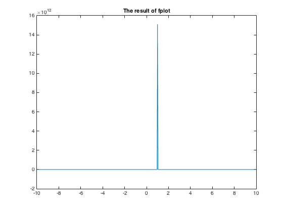
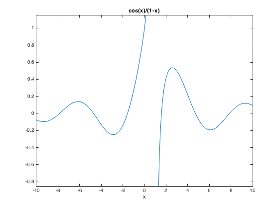
Clearly the two routines chose different values to bound the y coordinate! As a result, the fplot figure is misleading, since the function doesn't actually have a positive "spike" at x = 1, but rather an asymptote that approaches infinity in two different directions, as we can see in the ezplot figure. Let's change the y bounds to be -1 to 1 in the first figure (the one produced by fplot). Do this by bringing that window to the front and choosing the menu option Edit ❯ Axes Properties….

A window will pop up. The first thing to do is to select the tab labeled "Y Axis" near the bottom. Next, uncheck the Auto box, if it is checked. This will allow you to edit the text boxes next to "Y Limits." Replace the bounds with -1 and 1, and then press Enter. The result after rescaling is:

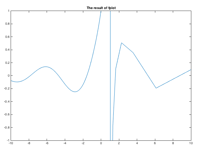
Notice how "rough" the graph still appears to be to the right of x = 1. This is probably due to it being originally graphed on such an extreme scale on the y-axis. Indeed, if we had known that we had wanted certain bounds on y beforehand, we could have included those bounds by entering fplot(f, [-10, 10, -1, 1]). Because this function has a vertical asymptote at x = 1, no matter what we do, fplot errantly draws a vertical line there.

Graph the function g(x) = ^sin(x)*x on the interval [-10,10] with fplot. Include the MATLAB code you used. Then paste the graph into your word document. To copy the graph, bring its window to the front and choose the menu option Edit ❯ Copy Figure.

Differentiation

MATLAB can compute derivatives of functions using the diff command. But first, we must declare what variables we are going to be using. Do this by the syms command:

To take the derivative of, say, sin(x), we can now type:

ans =
   cos(x)

MATLAB also allows us to differentiate functions of more than one variable. Let us use MATLAB to differentiate sin(x + 3y):

ans =
   cos(x + 3*y)

Note that MATLAB takes the derivative with respect to x and not y; by default, it will choose whichever symbol is closest to the letter X in the alphabet. If we wanted to take the derivative with respect to y instead, we would type

Compute the derivative of ln(sin(s)+cos(t)) with respect to t. Next, differentiate the same function with respect to s instead. Include the input and output in your Word document.

Solving ODEs Symbolically

MATLAB includes a helpful tool called dsolve that can produce symbolic solutions to basic differential equations. It is based on rather complicated algorithms for recognizing certain types of differential equations and solving them.

Consider the differential equation dy/dt = ky. You might have recognized this as a linear or separable equation, the solution of which is given by y = Ae^kt, where A is a constant equal to y(0).

Let's see how dsolve solves this equation by entering the following command:

The output is just what we expected (with C1 being the constant we called A). We can also add an initial condition to the equation, as follows:

The default independent variable in dsolve is t. Thus, if we want to have y as a function of, say, x, then we must specify that by typing dsolve('Dy=k*y', 'x'). Even if we enter a function of x into dsolve, it will not know that x is the independent variable unless we say so. Thus dsolve('Dy=2*x') returns not y = x^2 + C1 as you might expect, but rather 2*x*t + C1, because dsolve considers x to be a constant.

1. Consider the differential equation dy/dt = sin(t). Solve this equation by hand, without using MATLAB. [Hint: Just integrate both sides.] Write down the solution in your document.
2. Now use dsolve to solve the differential equation.
3. Using dsolve, solve the differential equation with initial condition y(0) = 3.

While dsolve may be useful at times, it has its limitations. For one, it cannot solve every equation. Also, the solution may be given in a form that is not useful to us.

Make up a differential equation that dsolve cannot solve. You should receive a warning message saying "explicit solution could not be found." or "Warning: Unable to find symbolic solution."

[Hint: You may need to experiment a little until you find such an equation. Try putting complicated functions of y and t on the right-hand side. You may find some of the functions used earlier in this lab useful here. You might also receive "Warning: Support of character vectors and strings will be removed in a future release. Use sym objects to define differential equations instead." You can just ignore this message or find the suggested way to apply dsolve with command help dsolve . We keep the old way as it's more straightforward.]

Copy and paste to your word document only the input and output for the equation you find that can't be solved. We do not need to see all of your experimentation.

For more information on dsolve, the help command should prove useful.

Conclusion: Submitting Labs

That's about it for Lab 1! At this point, your document should be ready to submit. In order to submit your document, you need to be enrolled in this course at Gradescope. This should happen automatically during the first week. However, if at the end of week 1 you do not yet have access to your class's MATLAB Gradescope page, you should contact your regular discussion section TA and explain the situation. Give them your name, UCSD email address, and PID, and they'll be able to add you to the course manually.

Please note that when submitting HWs on gradescope, you're required to assign correct pages to your problems. i.e. after you upload your pdf Gradescope will ask you to assign problems to specific pages of the pdf. If your solution to a problem consists of a few pages, you should include all of them. This will greatly help the graders find your work. Otherwise they have to scroll up and down to look for your answers and this is a lot of work since there are usually hundreds of HWs to grade. We should warn you that a few points will be deducted if you don't assign the pages correctly. (note: this happens after submiting the pdf)

To turn in your work, your document needs to be in PDF format. If you're using Word/ google docs, once you've saved your document, you can print as PDF or export it as a PDF in the File ❯ Export menu; alternatively, you can go to File ❯ Save As and choose "PDF" in the drop-down menu near the bottom. Once you've done this, open the Math 20D MATLAB course on Gradescope, find Assignment 1, and submit your PDF for this assignment.

After you have saved and uploaded your lab document, remember to log out of your PC.

A few final comments and warnings:

1. TAs are available for help during lab time, not via email the night before the assignment is due.
2. No emailing labs to TAs.

The future labs will contain most of the applications of differential equations to be found in Math 20D. These problems can take a little while to work out. Be warned that future labs will be longer than this one! Don't wait until the last minute to start.