Orthogonality & Least Squares

A basis for a vector space is a fine thing to have, but in this lab we're going to go a step further and convert bases into orthonormal bases. A basis where the vectors are orthonormal to each other lends itself nicely to various computations, such as finding vector coordinates with respect to the basis and projecting vectors onto various subspaces. Square matrices whose columns are orthonormal (called orthogonal matrices) extend this idea and have a lot of nice properties, some of which we'll explore in this lab.

When we have a bunch of experimental data, we often want to find a function that gives a good approximation of our data in order to build a model. Orthonormal bases will help us find these approximations using the method of least squares.

Orthogonality

We say that two vectors x and y are orthogonal when their inner product is zero, i.e.,

⟨x, y⟩ = x ∙ y = x^Ty = 0.

To compute inner products with MATLAB, you could enter

>> x'*y

Alternatively, use can use the command dot():

>> dot(x,y)

The name dot refers to "dot product," another name for the inner product of vectors.

Enter the following vectors into MATLAB.

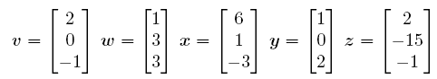
List all maximal orthogonal subsets of the above set. That is, group the vectors v, w, x, y, and z in as many ways as possible so that all the vectors in your group are orthogonal to each other and none of the vectors outside the group are orthogonal to all the vectors in the group. For example, the set {w, x} contains two vectors that are orthogonal to each other, and none of the other vectors are orthogonal to both of these at the same time. But this is only one example; there are more.

What is the maximum number of nonzero orthogonal vectors that you could possibly find in R³? What about Rⁿ? Explain.
Take the largest orthogonal subset and normalize all the vectors in that set as follows:
>> v = v/norm(v)
This code replaces v with itself divided by its size—so we get a vector pointing in the same direction but with length 1. The above code normalizes v, so you'll have to normalize the other vectors in your orthogonal subset as well, replacing v with the appropriate letter.

Store the resulting vectors in MATLAB as columns of a matrix W. Enter them in alphabetical order from left to right.

The matrix W we just computed is an orthogonal matrix: it is square, and its columns form an orthonormal set.

Calculate W^TW. What do you get? Why should we expect this result?
Enter the following vectors into MATLAB:

Compute the norm of b and the norm of Wb. What do you notice? Also compute the dot products ⟨a, b⟩ and ⟨Wa, Wb⟩.

One of the fundamental properties of orthogonal matrices is that they preserve norms of vectors and the standard inner product. (You can define orthogonal matrices as the ones with this property, in fact.)
The columns of W are linearly independent because the vectors are orthogonal, so W should clearly be invertible. Use inv(W) to compute the inverse of W, and then compare it to W^T. What do you observe?

Orthogonal matrices are incredibly important in geometry and physics. One reason for this is that orthogonal 2×2 matrices with positive determinant represent rigid motions of the plane about the origin; similarly, 3×3 orthogonal matrices with positive determinant give rigid motions of space about the origin. With negative determinants, you also allow reflections through a line or a plane. If you like, try to see geometrically why all distance-preserving linear transformations of the plane that keep the origin fixed must be either reflections or rotations (or both).

Orthogonal Projections

When we have two vectors pointing in different directions, we frequently want to divide one of the vectors into two pieces: one piece going in a direction parallel to the second vector, and one piece perpendicular to that direction. This gives us a way of writing the first vector in terms of the second one. We do this computation using orthogonal projections.

Hopefully, in the last section, you were able to see that the vectors v and w were not orthogonal. Suppose we want to find the orthogonal projection of v onto w—that is, the part of v traveling in the direction of w. Let's denote this vector by v̄. The projection formula says that

v̄ = (⟨v, w⟩/⟨w, w⟩)w

(Note that if w is normalized to length 1, then you need not divide by ⟨w, w⟩, since that is equal to 1 already.)

Here's a picture of what we're doing:

Find v̄, the orthogonal projection of v onto w. You can't enter v̄ as a variable name in MATLAB, so call it vbar instead. Also compute z = v - v̄, the component of v orthogonal to w. Then write v as the sum of these two vectors.
Use MATLAB to check that z is orthogonal to v̄. (Keep in mind that rounding errors in the computation might give you an answer that looks a little different from what you might expect.)

We've now seen how to project vectors onto other vectors. The idea behind projecting a vector onto a subspace instead is an easy extension of this method: we find an orthogonal basis for the subspace, project the vector onto each basis element, and then add up all the individual projections to form the orthogonal projection on the subspace.

Use MATLAB to find the projection of the vector (3, 3, 3)^T onto the subspace spanned by the vectors x and y (which we defined earlier in this lab).

The vectors x and y were already orthogonal, so in the last exercise we didn't have to compute an orthogonal basis. But if our basis vectors weren't orthogonal to each other, we'd have to modify them to make them orthogonal. In class you may have already seen the Gram–Schmidt process, which does exactly that.

The MATLAB command that performs the Gram–Schmidt process is called qr(). Given a matrix A, it performs an algorithm called QR factorization, returning two matrices: an orthogonal matrix Q whose columns are obtained from the columns of A using Gram–Schmidt; and an upper triangular matrix R such that A = QR.

Let's try to find an orthonormal basis for the subspace spanned by the vectors a and b we defined earlier. We start by defining a new matrix A whose columns are a and b.

>> A = [a b]

A =

    1	2
    1	0
    0	3

Next, we use the qr() command.

>> [Q,R] = qr(A)

Q =

    -0.7071     0.3015    -0.6396
    -0.7071    -0.3015     0.6396
     0          0.9045     0.4264

R =

    -1.4142     -1.4142
     0           3.3166
     0           0

You might notice that we only put two vectors (a and b) into A, and yet MATLAB gave us a matrix Q with three columns. In this case, the two orthonormal vectors we are looking for are the first two columns of Q. If we had supplied three vectors in R³ instead of just two, we'd use all three columns. Alternatively, we could enter the command [Q,R] = qr(A,0) to eliminate the extraneous columns. In any case, our orthonormal basis for the subspace spanned by a and b is

Now it's your turn to do this.

The set {(1, 2, 1)^T, (2, 1, 2)^T, (1, 1, 2)^T} is a basis for R³. As in the example above, turn it into an orthonormal basis. You should obtain an orthogonal matrix Q whose columns are the vectors obtained by performing Gram–Schmidt on this set.
Store the eigenvalues of Q in a vector v as follows:
>> v = eig(Q)
Then enter the following code:
>> norm(v(2))
This command tells MATLAB to find the absolute value of the second entry in the vector v, i.e., the absolute value of the second eigenvalue. Do the same for the third eigenvalue. What do you observe?

It is always the case that the eigenvalues of any orthogonal matrix will have absolute value 1. Suppose that you're working with a 3×3 orthogonal matrix T that happens to have determinant 1. The characteristic polynomial has degree three, and therefore it has a real root. The other two roots will be some unit complex number (including possibly 1 or -1) and its complex conjugate. The product of all three roots is supposed to be the determinant, and the product of the two complex roots is 1, so the real root must in fact be 1.

This means any orthogonal matrix T with determinant 1 must have 1 as an eigenvalue. If v is an eigenvector corresponding to this eigenvalue, then for any real number c, T(cv) = cTv = cv. So T fixes the entire axis on which v lies. And T is an orthogonal matrix, so it represents some rigid motion of space. Since it leaves one axis fixed, it must be a rotation around that axis! We've just deduced a remarkable theorem:

Euler's Theorem: A motion of a rigid body with one point fixed must be a rotation about some axis.

If you think about it, this is pretty striking. Imaging moving your phone around in your hands in such a way that the exact center of the phone always stays in the same place. You might be doing all sorts of crazy maneuvers with the phone as a whole, but as long as you keep that one point in the same spot, in the end your entire motion amounted to nothing more than a rotation around some axis.

Least Squares

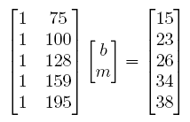
Now we'll turn to some more practical concerns. Suppose we're trying to study the relationship between temperature and pressure in a physical experiment. We attach a temperature and pressure sensor to a metal container. Starting at room temperature (75ºF), we slowly heat the air inside our container to 195ºF, recording temperature and pressure readings along the way. We get a total of five data points:

Temperature (ºF)	Pressure (lb/sq. in.)
75	15
100	23
128	26
159	34
195	38

Since we suspect the relationship here to be linear, we will be looking for a straight line with the equation y = mx + b, where y is the pressure, x is the temperature, m is the slope, and b is the y-intercept. We would like this line to pass through the data points we collected from the experiment. Plugging these data points into the equation for the line, we obtain the following system of equations:

b + 75m = 15
b + 100m = 23
b + 128m = 26
b + 159m = 34
b + 195m = 38

We'll attempt to solve this system. First, let's rewrite it in matrix form:

Unfortunately, this system doesn't have a solution, even though the underlying physical law really is a linear one. This is because it's impossible to have perfect accuracy when recording data. Instead of solving this system, we can instead try to find the closest linear solution. That is, we want to find the best fit line: the line that minimizes the sum of the squares of the distances from each data point to the line.

To simplify notation, let's assign names to the matrices and vectors of the above system.

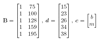
We're trying to find a vector c that minimizes the distance ‖Bc - d‖. Of course, we can never hope for this to be zero because Bc = d has no solutions. However, the equation Bc = proj_Vd, where V is the column space of B, does have a solution. That's because proj_Vd lies in the column space of B, and the linear transformation B hits every vector in its column space. The solution to this equation turns out to minimize the quantity ‖Bc - d‖. In the following exercise, we will solve the equation Bc = proj_Vd directly.

Enter the matrix B and the vector d into MATLAB. To compute proj_Vd, we must first find an orthonormal basis for V. For this, we use the qr() command:
>> [Q, R] = qr(B,0)
The columns of Q form an orthonormal basis for V. Let's give them their own names:
```
>> x = Q(:, 1)
>> y = Q(:, 2)
```
Now we're ready to compute proj_Vd. To do this, we add up the projections of d onto each element in our orthonormal basis, like so:
>> v = dot(x,d)*x + dot(y,d)*y
The resulting vector v here is proj_Vd. Remember to include all your input and output for this procedure in your write-up.
Now solve the equation Bc = proj_Vd = v by typing in the following:
>> c = B\v
Check that your answer is correct by entering
>> B*c - v
Make sure the answer is zero. (Keep in mind that MATLAB may return a very small number instead of zero due to rounding errors.)
Now let's compare the answer we just found to what MATLAB gives us when we run the built-in least squares algorithm named lscov. To use it, we must specify three parameters: the matrix B, the vector d, and a covariance matrix X, which we won't worry about in this course. Type in the following command:
>> cl = lscov(B, d, eye(5))
How does your answer to this part compare to your previous answer?

To illustrate the effectiveness of the least squares method, we'll plot our data points along with the best-fit line.

What is the equation of the best-fit line? (Remember that the equation of the line is y = mx + b, and the vector c we just obtained is equal to (b, m)^T.)
Use the equation of the line to calculate the pressure at the following temperatures: 35ºF, 170ºF, and 290ºF.
We can now plot the data points and our line to see visually if the approximation is good or not. Enter the following sequence of commands:
```
>> x = B(:,2);
y = d;
t = 0:1:300;
z = polyval([c(2);c(1)],t);;
plot(x,y,'x',t,z)
```

If you're curious, the command polyval() returns a polynomial of a specific degree with coefficients specified by a vector.

Conclusion

In this final lab, we've seen how orthogonality and the method of least squares can be harnessed to help us analyze experiments and find the best possible approximations for our data. These tools are essential to the process of building workable mathematical models in all kinds of applications.

Last Modified: 8 January 2017