Eigenvalues & Diagonalization

In this lab, we're going to learn how to use MATLAB to compute the eigenvalues, eigenvectors, and determinants of matrices. Then we'll use these new mathematical tools to revisit old problems from a new perspective.

Determinants

As you should be aware by now, there is a nice formula for calculating the determinant of a 2×2 matrix. Even the 3×3 case is not too hard. But as the size of a matrix increases, the determinant calculation gets much more complicated. This is where MATLAB comes in.

Start by entering the following two matrices in MATLAB:

To compute the determinants of these matrices, we use the command det():

>> det(A)

ans =
    76

>> det(B)

ans =
    48

Use MATLAB to compute the determinants of the matrices A+B, A-B, AB, A^-1, and B^T. (Recall that in MATLAB, B^T is written as B'.)
Which of the above matrices are not invertible? Explain your reasoning.
Suppose that you didn't know the entries of A and B, but you did know their determinants. Which of the above determinants would you still be able to compute from this information, even without having A or B at hand? Explain your reasoning.

In this class, we're interested in determinants mainly as a way to study the invertibility of matrices. When we use MATLAB for this purpose, we must be careful. Any computer program will introduce rounding errors, so a matrix that actually is invertible may appear to have zero determinant.

Enter the following matrix in MATLAB:

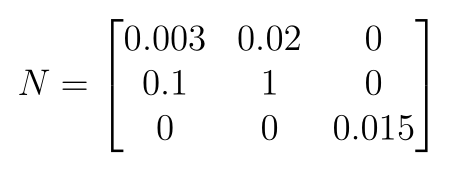
Use det() to calculate the determinant of N¹⁰⁰. Based on this information, do you think that N¹⁰⁰ is invertible?

Now compute the determinant of N. Calculate the determinant of N¹⁰⁰ by hand. Now would you reconsider your answer to the previous question? Explain.

What we've just seen in this exercise is an example of the sort of rounding error that computers can introduce.

Eigenvalues and Eigenvectors

As you may have already learned in class, an eigenvalue of a matrix A is a number λ such that the equation Av = λv has solutions other than the zero vector. Such a vector v is called an eigenvector corresponding to the eigenvalue λ. Generally, it's rather unpleasant to compute these eigenvalue and eigenvectors for a matrix by hand. Luckily, the MATLAB command eig() can perform this task for us.

Suppose we'd like to compute the eigenvalues of the matrix B we used earlier, and we want to store the eigenvalues in a vector b. We can do this using the following command:

>> b = eig(B)

b =
    1
    8
    3
    2

Thus we see that the eigenvalues are 1, 8, 3, and 2; there are four eigenvalues because our matrix is 4×4. (As an aside, note that we can quickly compute the determinant of B with this information: it's just the product of the eigenvalues.)

If we want to compute the eigenvalues and corresponding eigenvectors all in one step, we can simply use the following command:

>> [P,D] = eig(B)

P =

    1.0000   -0.1980   0.2357    0.9074
    0         0.6931  -0.2357   -0.1815
    0         0.6931   0.9428    0.3630
    0         0        0         0.1089


D =

    1 0 0 0
    0 8 0 0
    0 0 3 0
    0 0 0 2

The matrix P here has the eigenvectors of B as its columns, and the diagonal matrix D has the corresponding eigenvectors along the diagonal. This means, for instance, that the second column of P is an eigenvector for the eigenvalue 8, which is the second entry along the diagonal of D.

Let's quickly check this result. Enter the following command:

>> x = P(:,2);

This will store the second column of P as a new vector that we're calling x. Now enter

>> B*x - 8*x

If we've done everything correctly, we should get 0, since x is supposed satisfy the equation Bx = 8x.

Now let's explore one of the interesting properties of these eigenvalue and eigenvector matrices.

Enter the following matrix in MATLAB:
```
>>  V = [-8 6 -6 -30; 3 9 12 -10; 3 -6 -1 18; 3 0 4 7]			
```
Now use MATLAB to find the eigenvectors and corresponding eigenvalues of V. Assign them to matrices P and D, respectively.
Determine whether V is invertible by looking at the eigenvalues. Explain your reasoning.
Use MATLAB to evaluate P^-1VP. What do you notice?

Diagonalization

We've just seen an example of an important phenomenon called diagonalizability. We say that a matrix A is diagonalizable when we can find an invertible matrix P such that P^-1AP is diagonal. But this idea seems really arbitrary: why would anyone want to modify the matrix A like this just to make it diagonal?

To answer this question, let's think about the problem of raising A to a large power—100, say. This kind of computation is definitely useful; in a lot of real-world applications, you're interested in what happens when some process (represented mathematically by the matrix multiplication) is applied to some initial conditions (stored in a vector) over and over again. We could of course just multiply A by itself 100 times, but that makes for a lot of operations, even for a computer. It will take a long time, especially if A is large. However, diagonalization offers us a neat shortcut. If we could write A as PDP^-1, where D is a diagonal matrix, then we can do this:

A¹⁰⁰ = (PDP^-1)¹⁰⁰ = (PDP^-1)(PDP^-1)⋯(PDP^-1) = PD(P^-1P)D(P^-1P)⋯(P^-1P)DP^-1 = PD¹⁰⁰P^-1.

D¹⁰⁰ is much nicer than A¹⁰⁰ because in order to raise a diagonal matrix to a power, all you have to do is raise all of its entries to that power. This requires far fewer matrix multiplications.

Not every matrix is diagonalizable. In order to diagonalize an n×n matrix, we need to find n eigenvectors of that matrix that form a basis of Rⁿ. These n linearly independent eigenvectors form the columns of P, and then the entries of D are the matching eigenvalues. If we can't find a basis consisting only of eigenvectors, then the matrix isn't diagonalizable.

Theorem: If an n×n matrix has n distinct eigenvalues, then the matrix is diagonalizable.

Note that the converse is not true: some matrices are diagonalizable even though they don't have distinct eigenvalues. One example is the identity matrix, which is already diagonal and whose eigenvalues are all 1.

Enter this matrix in MATLAB:
>> F = [0 1; 1 1]
Use MATLAB to find an invertible matrix P and a diagonal matrix D such that PDP^-1 = F.
Use MATLAB to compare F¹⁰ and PD¹⁰P^-1.
Let f = (1, 1)^T. Compute Ff, F²f, F³f, F⁴f, and F⁵f. (You don't need to include the input and output for these.) Describe the pattern in your answers.
Consider the Fibonacci sequence {f_n} = {1, 1, 2, 3, 5, 8, 13…}, where each term is formed by taking the sum of the previous two. If we start with a vector f = (f₀, f₁)^T, then Ff = (f₁, f₀ + f₁)^T = (f₁, f₂)^T, and in general Fⁿf = (f_n, f_n+1)^T. Here, we're setting both f₀ and f₁ equal to 1. Given this, compute f₃₀.

The Fibonacci sequence we just saw is defined recursively: each term is given by a formula involving previous terms. By computing Fⁿ (which is done by computing PDⁿP^-1), we can actually derive an explicit formula for each term that doesn't require you to already know previous terms.

Electoral Trends Revisited

At the end of the last lab, we said we would revisit our election example once we had some more tools to work with. For your convenience, we've reprinted the information related to that example below:

In California, when you register to vote, you declare a party affiliation. Suppose we have just four political parties: Democrats, Republicans, Independents, and Libertarians. Party registration data is public, so we can track what fraction of the voters in each party switch to a different party from one election to the next. Let's say we look up Democratic Party registration data and discover the following: 81% of Democrats remain Democrats, 9% become Republicans, 6% re-register as Independents, and 4% become Libertarians. We can do the same kind of calculation for the other three parties and then organize our data into a table:

	Democrats	Republicans	Independents	Libertarians
Democrats	0.81	0.08	0.16	0.10
Republicans	0.09	0.84	0.05	0.08
Independents	0.06	0.04	0.74	0.04
Libertarians	0.04	0.04	0.05	0.78

In this table, we've put our results in the columns, so the numbers reflect the proportion of voters in that column's political party who switch to the party listed to the left. For example, the entry in the "Republicans" row and the "Independents" column tells us that 5% of Independents become Republicans each electoral cycle. We're going to assume that these numbers do not change from one election to the next—not a very realistic assumption, but good enough for our simple model.

Naturally, we want to use this data to predict the outcomes of future elections and the long-term composition of the electorate. Think of the table above as a matrix, which we will call P. Let D₀, R₀, I₀, and L₀ denote the current shares of the electorate held by Democrats, Republicans, Independents, and Libertarians, respectively. In the next election, these numbers will change according to P, as follows:

D₁ = 0.81 D₀ + 0.08 R₀ + 0.16 I₀ + 0.10 L₀ R₁ = 0.09 D₀ + 0.84 R₀ + 0.05 I₀ + 0.08 L₀ I₁ = 0.06 D₀ + 0.04 R₀ + 0.74 I₀ + 0.04 L₀ L₁ = 0.04 D₀ + 0.04 R₀ + 0.05 I₀ + 0.78 L₀

Let x_n be the vector (D_n, R_n, I_n, L_n)^T. This vector represents the party distribution after n electoral cycles; the first entry is the portion who are Democrats, the second the portion who are Republicans, and so on. The equations we just wrote out above show us that x₁ = Px₀. In general, x_n = Pⁿx₀.

You're going to need the matrix P and initial distribution vector x₀ from the exercise we did:

>> P = [0.8100 0.0800 0.1600 0.1000;
0.0900 0.8400 0.0500 0.0800;
0.0600 0.0400 0.7400 0.0400;
0.0400 0.0400 0.0500 0.7800]

>> x0 = [0.5106; 0.4720; 0.0075; 0.0099]

You'll also need your results from that exercise, so go ahead and redo it if you don't have your answers handy. (You don't need to include them in your write-up this time, however.) Your results probably seemed to stabilize as we went further into the future. Let's try to explain that mathematically.

For this exercise, we'll need to introduce the concept of limits. Many of you will have already seen limits in pre-calculus or calculus classes. A rough intuitive definition of limit is this: a limit is a number that a function "approaches" when the numbers you plug in to that function get close to a certain value. So if we say, "The limit of the function f(x) when x approaches 2 is 5," that means we can make f(x) as close as we like to the value 5 by choosing values for x that are closer and closer to 2.

You can also speak of limits of sequences of numbers: if we have a sequence {a_n}, to say that the limit of this sequence is L is to say that however close you ask me to get to L, I can find a term in the sequence so that all the subsequent terms are that close to L. Formally, the criterion is that for every positive number ε (no matter how small), there is an index N such that for each term x_n after x_N, the difference between L and x_n is less than ε.

Some sequences are easy to compute limits for. For example, consider the geometric sequence {r, r², r³, r⁴, …}. We can see what happens simply by checking how big r is. If |r| < 1, then the terms get smaller and smaller and eventually approach 0. If r = 1, then the sequence just stays at 1 forever. And if r > 1, the terms grow larger and larger, and we say that the limit is infinity.

Use MATLAB to find a matrix Q and a diagonal matrix D such that P = QDQ^-1.
Now recall that Pⁿ = QDⁿQ^-1. Find the limit as n tends to infinity of Dⁿ by hand; we'll call the resulting matrix L.
Using MATLAB, multiply L by Q and Q^-1 (on the appropriate sides) to compute P_∞, the limit as n tends to infinity of Pⁿ. Store the answer in a variable called Pinf.
Now use MATLAB to compute P_∞x₀. How does your answer compare to the results you saw in the second part of the exercise from last lab?
Make up any vector y in R⁴ whose entries add up to 1. Compute P_∞y, and compare your result to P_∞x₀. How does the initial distribution vector y of the electorate seem to affect the distribution in the long term? By looking at the matrix P_∞, give a mathematical explanation.

PageRank Revisited

Back in Lab 2, we discussed Google's PageRank algorithm for ranking websites using linking information stored in a linking matrix L. The version of the algorithm we presented worked well for our simple examples, but it turns out that Google doesn't solve the problem using the methods we implemented—our original method is too slow to handle extremely large linking matrices.

We want to find a quick way to solve the equation Lr = r even when the dimension of the linking matrix L is very large (and we expect L to be large because the web is huge). One thing we have going for us is that almost all the entries of L are going to be 0, since most websites don't link to most other websites. Our favorite technique for solving linear systems, Gaussian elimination, will mess this up: after only a few steps, a lot of the zero entries will be replaced with nonzero numbers. So we'd prefer to try something else. Here, we'll use a more elaborate version of the theorem we relied on before.

Theorem (Perron–Frobenius): For any matrix L whose entries are all nonnegative and whose columns each sum to one, the largest eigenvalue is 1. Moreover, for any vector r₀ with positive entries, the vector r_n = Lⁿr₀ approaches a nonnegative vector r that is a solution to the eigenvalue problem Lr = r.

Now we've recast the phenomenon behind PageRank as one involving eigenvalues, eigenvectors, and iteration of the matrix L (i.e., raising L to large powers). Specifically, if we take n to be large enough, then Lⁿr₀ will approach the solution we're looking for.

Consider the following linking matrix showing connections between the websites A, B, C, D, E, F, G, and H:

Enter this matrix into MATLAB with the command

>> L = [0,0,0,0,1,0,0,0;
0,0,0,0,0,0,0,1;
0,1/2,0,0,0,0,1,0;
1/2,0,1/2,0,0,0,0,0;
0,0,1/2,0,0,1,0,0;
1/2,0,0,0,0,0,0,0;
0,1/2,0,0,0,0,0,0;
0,0,0,1,0,0,0,0;]

Let e₀ = (1, 1, 1, 1, 1, 1, 1, 1)^T, and define e_n+1 = Le_n (which is the same as saying e_n = Lⁿe₀). Use MATLAB to compute e₁₀. How large must n be so that each entry of e_n changes by less than 1% when we increase n by 1? [Don't try to get an exact value, just try to get a value for n that's big enough.]
In the graph of the network of webpages represented by L, which vertices have an edge going out and pointing toward website C? Which vertices do the edges coming out of C point to? (Here, by graph we mean a collection of vertices and edges.)

If you find this PageRank algorithm interesting, you might try to answer the following question: what is the computation cost of solving Lr = r using iteration? More precisely, about how many operations are required to find r_n in this method? Multiplying a number by 0 and adding two numbers together each cost almost no time, so we just need to count how many times we have to multiply two nonzero numbers together.

What usually happens in practice for very large L is that the convergence of r_n to r is very quick, and so the size of n needed for decent accuracy often doesn't go up rapidly with the dimensions of L. This is very important because the dimensions of L for real websites will be on the order of hundreds of millions. Convergence is especially quick if our initial guess at the answer is good.

The type of iteration we've just seen is the basic idea behind solving many large-scale problems, not just PageRank. Methods like Gaussian elimination implemented in MATLAB are very reliable for matrices of modest size, but they take a long time when there are more than a few hundred variables. Iterative methods work well on large matrices with high probability, but they're not completely reliable—some matrices will mess them up.

Conclusion

We've now learned how to use MATLAB to compute determinants, eigenvalues, and eigenvectors, and we've used these tools to diagonalize matrices. We've also studied how these things can be applied to study fairly complex models using iteration.

Last Modified: August 2021