Matrix Algebra

---

We've seen how to use MATLAB to row-reduce matrices and solve linear systems; now we're going to use it to perform other basic matrix operations. In a sense, matrices are a bit like real numbers: we can add, subtract, and multiply them, provided they have appropriate dimensions. Some square matrices also have a multiplicative inverse. But there are a handful of striking differences. For example, when multiplying matrices, it is not generally true that AB = BA, and A² may be zero even when A is not the zero matrix. Keep these things in mind as you work through this lab.

Basic Matrix Operations

You've learned in class by now that we can add two matrices of the same dimensions by just adding the corresponding entries. The operator MATLAB uses for matrix addition is the simple plus sign +, the same one used for regular addition of numbers. If we enter the matrices

>> A = [1 2 3 4; 5 6 7 8]
>> B = [8 7 6 5; 4 3 2 1]

into MATLAB, we can then add them by typing

>> A+B

ans =
    9    9    9    9
    9    9    9    9

Matrix multiplication works as you would expect—you simply need the number of columns of the first matrix to be equal to the number of rows of the second one. For example, we could enter the following matrices into MATLAB:

>> C = [1 2; 1 0]
>> D = [0 1; 1 1]

Now we can multiply them:

>> C*D

ans =
    2    3
    0    1

We can also exponentiate matrices (as in A^3). Lastly, we can ask MATLAB to compute the tranpose of a matrix with an apostrophe ('):

>> C'

ans =
    1    1
    2    0

Matrix Inversion

One of the key differences between matrix multiplication and multiplication of real numbers is in the existence of multiplicative inverses. If x is a nonzero real number, then there's always another number (namely ¹⁄_x) that you can multiply by x to get the multiplicative identity (1). With matrices, we'd like to do the same thing: given a matrix A, we want to find another matrix B such that AB = BA = I, where I is an identity matrix.

Just by looking at the condition AB = BA = I, we can see that A and its inverse B have to be square matrices of the same dimension. Unfortunately, even square nonzero matrices can fail to have an inverse. If an inverse exists, we say that A is invertible (or sometimes non-singular); otherwise, we say it is non-invertible (singular).

The MATLAB command inv finds the inverse of a matrix if it exists.

Logistics: Route Planning

Suppose we have a business operating in five cities around the Pacific Rim: San Diego, Los Angeles, Tokyo, Shanghai, Manila, and Seattle. We are interested in counting the number of ways we can travel from one city to another with at most n stopovers. We look up all the direct flights and put them in a table:

	Destination
San Diego	Los Angeles, Seattle
Los Angeles	San Diego, Tokyo, Shanghai, Manila, Seattle
Tokyo	Los Angeles, Shanghai, Manila, Seattle
Shanghai	Los Angeles, Tokyo, Manila, Seattle
Manila	Tokyo, Shanghai
Seattle	San Diego, Los Angeles, Tokyo, Shanghai

Doing that last exercise by hand is a pain because there are so many cases to check, and this is a relatively simple example. If we want to do this efficiently, linear algebra is the perfect tool. We'll start by encoding the data from our table into what's called an adjacency matrix.

The first step is to number our cities in the order they are listed: San Diego is 1, LA is 2, and so on. We now determine the entries of our adjacency matrix, which we will call A, using the following rule: if there is a flight from city i to city j, then the entry A_ij is set to be 1. Otherwise, we set that entry to be 0. We will also set all of the diagonal entries to be 0, since you can't take a flight from a city to itself. This procedure gives us the following matrix A:

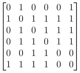
What's neat about this is that the powers of A have useful information too. For example, take the entry (A²)₃₆ (i.e., the entry of A² in the third row and sixth column). We compute this as

(A²)₃₆ = A₃₁A₁₆ + A₃₂A₂₆ + A₃₃A₃₆ + A₃₄A₄₆ + A₃₅A₅₆ + A₃₆A₆₆

Let's look at the terms here: A_3kA_k6 is 1 if and only if both A_3k and A_k6 are 1. This means we get a 1 for the k^th term if and only if we can fly from Tokyo (city 3) to city k and from city k to Honolulu (city 6). Thus, (A²)₃₆ counts the number of ways to fly from Tokyo to Honolulu with exactly one stop. Similar reasoning shows that the number of ways of flying from city i to city j with exactly n stops is just (Aⁿ⁺¹)_ij .

As you may have realized, the method we've just used counts silly trips like Manila → Shanghai → Seattle → Shanghai → Seattle as a trip with three stops although few people would do that in real life. So the number may seem large. User beware!

Political Science: Electoral Trends

We've already seen how linear algebra can be used to evaluate simple social networks. Now we're going to look at another kind of sociological situation, where we'll try to use matrices to model future population dynamics.

In California, when you register to vote, you declare a party affiliation. Suppose we have just four political parties: Democrats, Republicans, Independents, and Libertarians. Party registration data is public, so we can track what fraction of the voters in each party switch to a different party from one election to the next. Let's say we look up Democratic Party registration data and discover the following: 81% of Democrats remain Democrats, 9% become Republicans, 6% re-register as Independents, and 4% become Libertarians. We can do the same kind of calculation for the other three parties and then organize our data into a table:

	Democrats	Republicans	Independents	Libertarians
Democrats	0.81	0.08	0.16	0.10
Republicans	0.09	0.84	0.05	0.08
Independents	0.06	0.04	0.74	0.04
Libertarians	0.04	0.04	0.05	0.78

In this table, we've put our results in the columns, so the numbers reflect the proportion of voters in that column's political party who switch to the party listed to the left. For example, the entry in the "Republicans" row and the "Independents" column tells us that 5% of Independents become Republicans each electoral cycle. We're going to assume that these numbers do not change from one election to the next—not a very realistic assumption, but good enough for our simple model.

Naturally, we want to use this data to predict the outcomes of future elections and the long-term composition of the electorate. Think of the table above as a matrix, which we will call P. Let D₀, R₀, I₀, and L₀ denote the current shares of the electorate held by Democrats, Republicans, Independents, and Libertarians, respectively. In the next election, these numbers will change according to P, as follows:

D₁ = 0.81 D₀ + 0.08 R₀ + 0.16 I₀ + 0.10 L₀
R₁ = 0.09 D₀ + 0.84 R₀ + 0.05 I₀ + 0.08 L₀
I₁ = 0.06 D₀ + 0.04 R₀ + 0.74 I₀ + 0.04 L₀
L₁ = 0.04 D₀ + 0.04 R₀ + 0.05 I₀ + 0.78 L₀

Let x_n be the vector (D_n, R_n, I_n, L_n)^T. This vector represents the party distribution after n electoral cycles; the first entry is the portion who are Democrats, the second the portion who are Republicans, and so on. The equations we just wrote out above show us that x₁ = Px₀. In general, x_n = Pⁿx₀.

Conclusion

Hopefully, this lab has given you a little more intuition for the properties of matrices and their differences from real numbers. In the last exercise, you've also made some interesting observations about what happens when we apply the same matrix to a vector over and over again. In the next lab, we'll develop more mathematical tools to help explain this behavior.

---

Last Modified: 8 January 2017