Systems of Linear Equations
You have already encountered linear equations many times in your career as a student. Most likely, the very first equation you had to solve was linear. This kind of equation is extremely simple, yet systems of multiple linear equations are of immense important in a huge variety of mathematical, scientific, and sociological fields. Math 18 is probably your first systematic study of linear equations, and in this lab we're going to see how we can use MATLAB to solve them. We will also learn about a very useful application of this kind of mathematics to economics and computer science.
Solving Linear Systems
By now we have seen how a system of linear equations can be transformed into a matrix equation, making the system easier to solve.
The system
2x1 - 1x2 + 1x3 = 8
1x1 + 2x2 + 3x3 = 9
3x1 + 0x2 - x3 = 3
can be written in the following way:

Now, by augmenting the matrix with the vector on the right and using row operations, this equation can easily be solved by hand. However, if our system did not have nice integer entries, solving it by hand using row reduction could become very difficult. MATLAB provides us with an easier way to get an answer.
A system of this type has the form Ax = b, so we can enter these numbers into MATLAB using the following commands:
>>A = [2 -1 1; 1 2 3; 3 0 -1]>>b = [8; 9; 3]
Notice that for the column vector b, we include semicolons after each entry to ensure that the entries are on different rows. If instead we had typed
>>b = [8 9 3]
we would have gotten a row vector, which is not the same thing. Now that we've defined A and b, the command
x = A\b
will find the solution to our equation Ax = b if it exists. In this case, MATLAB tells us
x =
   2.0000
  -1.0000
   3.0000
Please take care in entering the command A\b. It has a backslash (\), not a forward slash (/).
Consider the system of equations
2x1 + 1x2 + 6x3 = 1
1x1 + 0x2 + 3x3 = 2
-3x1 + 2x2 -7x3 = 3
Convert this system of equations into a matrix equation of the form Cx = d. Solve it by hand, and record your solution in your document.
-
Enter the matrix C and the column vector d into MATLAB, and use the command
>>x = C\dto check your solution.
-
We would expect to get the column vector d in MATLAB if we ran the command
>>C*x, right? In other words,C*x-dshould be zero. Enter this expression into MATLAB:C*x-dInclude the input and output.
There are drawbacks to using the command x = C\d, unfortunately. Let's explore them now.
Consider the system of equations
-10x1 + 5x2 = 0
6x1 - 3x2 = 0
As you did in the previous exercise, enter the corresponding matrix C and column vector d into MATLAB. Then type in
>>x = C\d
Note the strange output. Include it in your write-up. Now go ahead and solve this system by hand. How many free variables do you have in your solution? Based on your answer, can you explain why you got the error message when trying to use the command x = C\d?
To deal with the case of inconsistent systems or systems with infinitely many solutions, it may sometimes be better to simply use MATLAB to row-reduce your matrix and then read off the solutions yourself. Luckily, MATLAB has a command that performs Gaussian elimination for you.
Consider the following homogeneous system of equations:
2x1 + 0x2-3x3 = 0
4x1 + x2 + 2x3 = 0
2x1 + x2 + 5x3 = 0
Enter the corresponding matrix C and column vector d into MATLAB. Now we want to perform row reduction on the augmented matrix [C | d]. The command that performs row reduction in MATLAB is rref (the name stands for "reduced row echelon form"). Type in
>> rref([C d])

ans =

     1.0000         0   -1.5000         0
         0    1.0000    8.0000         0
         0         0         0         0
Recall from class that we can use this row-reduced form to see that x1 = 1.5x3 and that x2 = -8x3. Here, x3 is the free variable, and we can choose whatever value we want for it; once we do that, the other two variables are fixed. For instance, if we pick x3 = 2, then x1 = 3 and x2 = -16. There are infinitely many solutions because there are infinitely many choices for the value of x3, but they all follow this pattern.
Consider the homogeneous system of equations
x1 - 3x2 + 2x3 = 0
-2x1 + 6x2 - 4x3 = 0
4x1 - 12x2 + 8x3 = 0
By using the rref command, write down the general solution to this system of equations. How many free variables are required?
Now that we've seen MATLAB's basic tools for solving linear systems, let's turn to some applications.
Economics: Leontief Models
Wassily Leontief (1906-1999) was a Russian-born American economist who, aside from developing highly sophisticated economic theories, enjoyed trout fishing, ballet, and fine wines. He won the 1971 Nobel Memorial Prize in Economics for his work in creating mathematical models to describe various economic phenomena. In the remainder of this lab we will look at a very simple special case of his work called a closed exchange model. There are two basic assumptions:
- Everyone exclusively buys from and sells to the central pool (i.e., there is no outside supply or demand).
- Everything produced is consumed.
With these assumptions and some data about how the goods are consumed, we can compute exactly what price each good should have for everyone in the community to survive.
To see how this works, let's suppose there's a small country town with only five residents: a farmer, a tailor, a carpenter, a coal miner, and Slacker Bob. The farmer produces food; the tailor, clothes; the carpenter, housing; the coal miner, energy; and Slacker Bob makes moonshine, half of which he drinks himself. The following table lists what fraction of each good our five residents consume:
| Food | Clothes | Housing | Energy | Alcohol | |
|---|---|---|---|---|---|
| Farmer | 0.25 | 0.15 | 0.25 | 0.18 | 0.20 |
| Tailor | 0.17 | 0.28 | 0.18 | 0.17 | 0.10 |
| Carpenter | 0.22 | 0.19 | 0.22 | 0.22 | 0.10 |
| Miner | 0.20 | 0.15 | 0.20 | 0.28 | 0.15 |
| Slacker Bob | 0.16 | 0.23 | 0.15 | 0.15 | 0.45 |
So for example, the carpenter consumes 22% of all food, 19% of all clothes, 22% of all housing, 22% of all energy, and 10% of all the moonshine.
The columns in this table all add up to 1. Explain why.
Now, let f, t, c, m, and b denote the incomes of the farmer, tailor, carpenter, miner, and Bob, respectively. Note that each of these quantities represents not only the gross incomes of each of our citizens but also the total cost of the goods they sell. So for example, f is the farmer's income and also is the cost of all the food. If the farmer produces $100 worth of food, then his income will also be $100, since all of this food gets purchased and all the revenue goes to the farmer.
We want to price the goods so that everyone earns enough money to pay for all the goods they consume. To do that, we need to satisfy the following five equations:
0.25f + 0.15t + 0.25c + 0.18m + 0.20b = f
0.17f + 0.28t + 0.18c + 0.17m + 0.10b = t
0.22f + 0.19t + 0.22c + 0.22m + 0.10b = c
0.20f + 0.15t + 0.20c + 0.28m + 0.15b = m
0.16f + 0.23t + 0.15c + 0.15m + 0.45b = b
Explain where this system of equations came from and what it means. (What do the left-hand side and the right-hand side of each equation represent?)
Let's denote the column vector (f, t, c, m, b)T by p. Let C be the coefficient matrix of the above system. We can now rewrite that system as Cp = p, or equivalently,
Cp - p = Cp - Ip = (C - I)p = 0
where I is the 5×5 identity matrix.
Enter the matrices C and I into MATLAB.
>>C = [0.25 0.15 0.25 0.18 0.20; 0.17 0.28 0.18 0.17 0.10; 0.22 0.19 0.22 0.22 0.10; 0.20 0.15 0.20 0.28 0.15; 0.16 0.23 0.15 0.15 0.45]>>I = eye(5)
The command eye(n) used here creates an n×n matrix with ones on the diagonal and zeros elsewhere.
-
Use MATLAB to row-reduce the augmented matrix [C - I | 0], and write down the general solution to (C - I)p = 0.
-
What are highest- and lowest-priced commodities in this model community? List the inhabitants in order of income, from lowest to highest. If our friend Bob sells $40,000 in moonshine per year, what are the gross incomes for the rest of the inhabitants?
Computer Science: Web Search
Here's a basic problem: in a particular group of people, who is the most popular?
One possible approach for answering this question is to ask everyone in the group to list their friends in that group. (This is a dangerous experiment—do not try it in your own social groups!) Suppose we're interested in a group of four people: June, Carlos, Meichen, and Felix. We will nickname them J, C, M, and F, respectively. We ask them to identify their friends, and they respond as follows:
| June | C, M |
|---|---|
| Carlos | J, M, F |
| Meichen | J, C, F |
| Felix | J, M |
We could represent this data in a 4×4 table of zeros and ones, where a 1 says that the person listed in the top row considers the person named on the left to be a friend:
| June | Carlos | Meichen | Felix | |
|---|---|---|---|---|
| J | 0 | 1 | 1 | 1 |
| C | 1 | 0 | 1 | 0 |
| M | 1 | 1 | 0 | 1 |
| F | 0 | 1 | 1 | 0 |
This really just amounts to a 4×4 matrix. Now, we could look at this table, count up the number of times someone is listed as a friend, and declare that to be the measure of someone's popularity. But the problem with that approach is that some people will tend to list everyone they know, and others will write down only their closest friends. If we try to score people this way, the former type of person will have outsized influence on the result.
Here's an alternate approach. We'll try to account for quality of friendship by assuming that it's better for a widely-liked person to think of you as a friend. Conversely, if someone whom nobody else likes considers you a friend, that doesn't make you popular.
To account for the problem we've identified, we'll normalize the lists of friends, dividing each column in our matrix by the number of people in it.
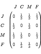
We shall call this the linking matrix and shall denote it by L.
With this data, we're going to assign to each person a number that we'll call their popularity: rJ, rC, rM, and rF. Combined, these numbers give the popularity vector
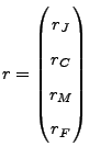
for the group. For our method, we will define popularity as follows:
A person's popularity is the weighted sum of the popularity of people who reference that person.
This looks like a circular definition, because we're defining popularity in terms of other people's popularity. But we can explain what the weights are and see how this is going to work by just writing out one of the equations:
rJ = 1⁄3 rC + 1⁄3 rM + 1⁄2 rF
This equation seems reasonable when we consider that June represents one third of Carlos's friends, so she is "rewarded" with one third of his popularity. She's also a third of Meichen's friend group, and she's fully half of Felix's list. If we wrote out all four of these equations and then converted to matrix-vector form, we would get exactly the equation
Lr = r
which is the same as
(L - I)r = 0
where I is the 4×4 identity matrix. If we can solve this equation, that gives us the relative popularity of all four of our subjects. To do that, we enter L into MATLAB and then use the command
>> rref([L-eye(4)])

ans =
   1.0000        0        0  -1.5000
        0   1.0000        0  -1.3125
        0        0   1.0000  -1.6875
        0        0        0        0
We can see here that we have one free variable. If we (arbitrarily) set rF = 1, then we'll get rJ = 1.5, rC = 1.3125, and rM = 1.6875. Thus, Meichen is the most popular, followed by June, then Carlos, and finally Felix.
PageRank
Some graduate students at Stanford got the idea that this sort of method could be used to rank a group of web pages. You type in some key words, and the software identifies a vest collection of webpages containing those words. Most of these will be garbage, as far as you are concerned. The challenge, then, is to automatically find a few good (popular) webpages.
The founders of Google had the software look at each webpage w in the set of results and determine which other webpages w links to. Thus, each webpage produces a vector of zeros and ones, just as we saw above with the students' lists of friends. Next, the algorithm builds a matrix whose columns are the normalized versions of these vectors. From there, it proceeds roughly the same way we did in the popularity problem. Google uses special methods to compute popularity very quickly, and then it lists for you the results from highest to lowest popularity.
This all sounds like a good plan, but you have to be sure of a few things before you can build a company out of this idea.
- Does the equation Lr = r always have a solution? (Is there anything you've seen in class so far to make you think it might not?)
- Will a solution have nonnegative entries? Negative solutions might be hard to interpret.
- Is the solution unique? If not, we will have conflicting rankings?
Fortunately, the founders of Google knew a handy theorem.
Theorem (Perron–Frobenius): For any matrix L whose entries are all nonnegative and whose columns each sum to one, the equation Lr = r has a nonnegative solution.
Thus the Perron–Frobenius theorem says there is always a solution to the popularity problem. We won't go into details on this, but the theorem also tells us that the solution is usually unique, and it explains the circumstances when it is not.
In the late 1990s, the leading search engine was Yahoo; they employed warehouses full of people to look at web pages and manually grade them. By using this simple mathematical model (plus a few bells and whistles), Google quickly displaced Yahoo. The ranking you just saw is often called PageRank after Larry Page, co-founder of Google, who in a few years became one of the ten wealthiest Americans. The extremely basic problem we just saw is the core of the rapidly-growing field of network analysis.
Now it's time for a little practice with the PageRank algorithm.
Suppose that we have five websites: A, B, C, D, and E. Let's also suppose that the links between the sites are depicted in the graph below:

Here, the arrow pointing from C to D means that there is a hyperlink on site C that takes you to site D. Recall that the third column represents the edges from C and thus the (4,3) component of the linking matrix is 1 before the normalization since there is an edge from C to D. For small sets of objects, graphs like this one are a convenient way to depict connections.
-
Create a linking matrix L containing the information of which site links to which, just as we did in the popularity example. Remember to normalize, and be sure that your input is exact. (For example, make sure you enter 1/3 instead of 0.3333—this is important for the next part of this exercise, since our columns must sum to 1.) Include all input and output from MATLAB.
-
Use the
rrefcommand to find all solutions x to the matrix equation (L - I)x = 0. Include all input and output from MATLAB. If you get an error message, be sure to double-check your answer for the first part of this exercise. -
Which website has the highest PageRank? Explain your answer, especially in light of any negative numbers that may have appeared in your solutions. List the remaining websites in decreasing PageRank order.
Obviously, the examples we have worked with so far are grossly simplified. In practice, the linking matrix is often huge, and we need to figure out a fast way to solve Lr = r for matrices of enormous size. Gaussian elimination on big matrices takes an extremely long time. Luckily, most entries of L end up being zero. Such a matrix is called a sparse matrix, and one major branch of mathematics is devoted to solving problems with sparse matrices. We will glimpse one of these methods in a later assignment.
Conclusion
Systems of linear equations are very basic mathematical objects that nevertheless show up in many interesting places. We've seen just two such applications today. Because the linear systems that show up in real-world settings tend to be absolutely enormous, it's impractical to work with them by hand. Computer programs like MATLAB are indispensable tools for people who must interact with such systems in their work.
Last Modified: 8 January 2017